Flexibility and sensitivity in gene regulation out of equilibrium

Abstract

Cells adapt to environments and tune gene expression by controlling the concentrations of proteins and their kinetics in regulatory networks. In both eukaryotes and prokaryotes, experiments and theory increasingly attest that these networks can and do consume biochemical energy. How does this dissipation enable cellular behaviors forbidden in equilibrium? This open question demands quantitative models that transcend thermodynamic equilibrium. Here, we study the control of simple, ubiquitous gene regulatory networks to explore the consequences of departing equilibrium in transcription. Employing graph theory to model a set of especially common regulatory motifs, we find that dissipation unlocks nonmonotonicity and enhanced sensitivity of gene expression with respect to a transcription factor's concentration. These features allow a single transcription factor to act as both a repressor and activator at different concentrations or achieve outputs with multiple concentration regimes of locally enhanced sensitivity. We systematically dissect how energetically driving individual transitions within regulatory networks, or pairs of transitions, generates a wide range of more adjustable and sensitive phenotypic responses than in equilibrium. These results generalize to more complex regulatory scenarios, including combinatorial control by multiple transcription factors, which we relate and often find collapse to simple mathematical behaviors. Our findings quantify necessary conditions and detectable consequences of energy expenditure. These richer mathematical behaviors-feasibly accessed using biological energy budgets and rates-may empower cells to accomplish sophisticated regulation with simpler architectures than those required at equilibrium.

Keywords: biophysics; gene regulation; nonequilibrium; transcription.

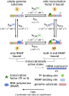
Fig. 1.

Structure of a fundamental gene-regulatory motif. A square cycle of four-states emerges when up to two molecules (such as a transcription factor $X$ and polymerase $P$) can bind to a common substrate (say a genome). Output observables $⟨r⟩$ are linear combinations of the state probabilities; for instance, mRNA production scales with the probabilities of transcriptionally active states where polymerase is bound to the genome (states $P$ and $\mathit{XP}$). These outputs vary with the control parameter $[X]$, here schematized as the concentration of a transcription factor. (Numerical values of rate constants underneath edges are biologically plausible values, as inferred in SI Appendix, section 2B).

Fig. 2.

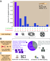
Incidence of regulatory architectures for transcription, where a square cycle’s response is common. (A) Regulatory architectures reported in E. coli, organized by the numbers of activating and repressing transcription factors associated with each regulated promoter, according to data in the RegulonDB database (19) release 11.2. Over half of these regulated promoters are reported to be regulated by the most common architecture of a single transcription factor (purple bars) and thus can be described by a square graph of states (Fig. 1). Less common network architectures with multiple transcription factors form hypercubic state spaces whose complete responses are analyzed in SI Appendix. (B) While larger binding networks can generically show more complex regulatory responses than the square cycle, simpler topologies and responses result from restrictions like overlapping binding site (SI Appendix, section 3D). Over half of all nontrivial transcriptionally potent derivative networks formed by up to three transcription factors show a response that resembles the square graph with respect to at least one transcription factor. (C) Transcriptional regulation by DNA looping accomplishes distinct responses, whose properties are analyzed algebraically and numerically in SI Appendix.

Fig. 3.

Nonequilibrium response of the four-state fundamental transcriptional motif. (A) An example of a spanning tree (rooted in state XP) like those that define steady-state probabilities via the Matrix Tree Theorem. (B) All 16 directed, rooted spanning trees of the four-state cycle in 1(A): trees are grouped by the root state (in columns) and by how many participating edges depend on the control parameter $X$ (in rows). As guaranteed by the Matrix Tree Theorem, the steady-state probability of any state—in or out of equilibrium—is given by the sum of the weights of these spanning trees, introducing up to a quadratic dependence in $X$ in any output, as represented by Eq. 1. (C–E) Three universal output behaviors (regulatory shape phenotypes) can result from this architecture. A monotonic “equilibrium-like” output (C) manifests a Hill-like or MWC-like response, behavior familiar from equilibrium thermodynamic models. However, exclusively out of equilibrium, new multiply-inflected regulatory shape phenotypes become possible. Under drive, outputs can (D) vary nonmonotonically and reach two inflection points with the control parameter; or show three inflection points and vary monotonically (E). These richer phenotypes show a wider set of properties that characterize each curve: These include the “leak” value of the observable when the control variable is absent (${⟨r⟩}_0=⟨r⟩([X]=0)$, in orange; the saturation asymptotic limit as the control variable is maximally present (${\langle r\rangle }_{\infty }=\underset{[X]\to \infty }{\lim }\langle r\rangle$; in light blue); the observable’s values at intermediate plateau regions (${⟨r⟩}_{\ast }$; in red); and slopes 1 and 2 at inflection points ${[X]}_1$ and ${[X]}_2$ when they are defined (in green and purple, respectively).

Fig. 4.

Global bounds, in or out of equilibrium, restrict maximal (normalized) response sensitivity (with respect to input concentrations $[X]$ on a log scale). The normalized responses $\frac{⟨r⟩-{⟨r⟩}_{\text{min}}}{{⟨r⟩}_{\text{max}}-{⟨r⟩}_{\text{min}}}$ are plotted near points of inflection that maximize slope, separated by shape phenotype. When the output has one inflection point (Left), the maximal sensitivity is bounded between a minimum of $0.16$ (blue line) and a maximum of 1/2 (red line) for any set of rate values or any dissipation; this subsumes the equilibrium case, whose normalized sensitivity is fixed at 1/4 (black dotted line). When the output has two inflections (Middle), the maximal sensitivity is bounded between 1/4 and 1/2. When the output has three inflections (Right), the maximal sensitivity is bounded between 1/8 and 1/4.

Fig. 5.

Systematically breaking detailed balance edge-by-edge. (A) Example of how spending energy to modify a single rate (here, $k_{\mathit{XS}}$)—while the seven other rates remain fixed—changes the response curve away from default equilibrium behavior (pale yellow curve labeled “0” net drive and outlined in black). Responses from rate values larger than (or smaller than) at equilibrium are shown in increasingly red (or blue) colors, respectively; curves are also labeled with the numerical values of the net drive that generated them in $k_{B}T$ units (positive for an increase; negative for a decrease). Each curve’s resulting inflection points are marked by yellow, orange, or pink markers, denoting one to three inflection points (respectively), and summarized in the associated one-dimensional (shape phenotypic) phase-diagram with the same colors on the Right. Inset: the position of the final inflection point $maxln{[X]}^{\ast }/{[X]}_0$ versus net drive (power law exponent is ∼1). (B) Another representative behavior is displayed when $k_{X,XP}$ is instead the rate varied. Inset: the saturation ${⟨r⟩}_{\infty }$ versus net drive (power law exponent is ∼1). (C) Summary of how all eight rates respond to energy expenditure to realize different regulatory shape phenotypes. Below, stem plots give precise values of each default rate constant at equilibrium. (These rates satisfy initial “broken symmetries” that violate the conditions in Eq. 5 by default, facilitating more ready access to nonmonotonicity. SI Appendix, section 2K documents the impact of departing from different default starting rates that instead satisfy Eq. 5, in addition to the impacts of driving all other edges.) (Here, the reference concentration scale setting the horizontal offset of the concentration axis is ${[X]}_0\equiv 1\text{nM}$).

Fig. 6.

Breaking detailed balance along two edges unlocks higher sensitivity and multiply-inflected outputs with smaller drive than required for breaking detailed balance along single edges. (A) Adjusting the rate pair $(k_{\mathit{SX}},k_{\mathit{PS}})$—while fixing the other six rates at their default biological values at equilibrium (of Figs. 3A and 5C’s stem plot)—varies the number of inflection points (light yellow: one inflection, orange: two inflections, pink: three inflections), in a 2D analog of Fig. 3. Specifically, this rate pair illustrates a case where nonmonotonic two-inflection curves can be reached with only an infinitesimal net drive. (B) In contrast, when tuning $(k_{\mathit{XS}},k_{\mathit{SX}})$, a finite minimum drive is needed to access nonmonotonicity; numerical sampling reveals that this total drive is the same as required while only tuning one edge at a time. (C) Maxima of raw slope $d⟨r⟩/dln[X]/{[X]}_0$ over the same modulations (axes) of the rate pair $(k_{\mathit{SX}},k_{\mathit{PS}})$ shown in (A), with slope-maximizing rates within the permissible rate space indicated with a circle. ${[X]}_0\equiv 1\text{nM}$ is a reference concentration. (D) Overlaying the same positions of maximal slope for all twenty-eight rate pairs emphasizes that optimal slopes are found at the boundary of the permissible rate space. Marker colors reflect the maximal slope achieved for each rate pair. Panel (E) summarizes the behavior of panel (D) by representing each optimal rate pair value with two important natural parameters: the net drive $\mathrm{\Delta }\mu /k_{B}T$ (either the log ratio or log product of each rate’s difference from their equilibrium starting values, depending on the relative (counter)clockwise orientation of the rates in a pair); and the net total distance in rate space between the optimal values and their starting values, $D\left(ln\frac{k_{\mathit{mn}}}{k_{m{n}^{\mathit{eq}}}},ln\frac{k_{\mathit{ij}}}{k_{i{j}^{\mathit{eq}}}}\right)\equiv \sqrt{{\left(ln\frac{k_{\mathit{mn}}}{k_{m{n}^{\mathit{eq}}}}\right)}^2+{\left(ln\frac{k_{\mathit{ij}}}{k_{i{j}^{\mathit{eq}}}}\right)}^2}$.

References

1. Morrison M., Razo-Mejia M., Phillips R., Reconciling kinetic and thermodynamic models of bacterial transcription. PLoS Comput. Biol. 17, e1008572 (2021). - PMC - PubMed
1. Grah R., Zoller B., Tkačik G., Nonequilibrium models of optimal enhancer function. Proc. Natl. Acad. Sci. U.S.A. 117, 31614–31622 (2020). - PMC - PubMed
1. Wong F., Gunawardena J., Gene regulation in and out of equilibrium. Annu. Rev. Biophys. 49, 199–226 (2020). - PubMed
1. Coulon A., Chow C. C., Singer R. H., Larson D. R., Eukaryotic transcriptional dynamics: from single molecules to cell populations. Nat. Rev. Genet. 14, 572–584 (2013). - PMC - PubMed
1. Shelansky R., Boeger H., Nucleosomal proofreading of activator-promoter interactions. Proc. Natl. Acad. Sci. U.S.A. 117, 2456–2461 (2020). - PMC - PubMed
Substances
LinkOut - more resources