Input/Output Relationships for the Primary Hippocampal Circuit

Abstract

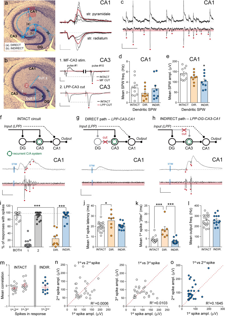
The hippocampus is the most studied brain region, but little is known about signal throughput-the simplest, yet most essential of circuit operations-across its multiple stages from perforant path input to CA1 output. Using hippocampal slices derived from male mice, we have found that single-pulse lateral perforant path (LPP) stimulation produces a two-part CA1 response generated by LPP projections to CA3 ("direct path") and the dentate gyrus ("indirect path"). The latter, indirect path was far more potent in driving CA1 but did so only after a lengthy delay. Rather than operating as expected from the much-discussed trisynaptic circuit argument, the indirect path used the massive CA3 recurrent collateral system to trigger a high-frequency sequence of fEPSPs and spikes. The latter events promoted reliable signal transfer to CA1, but the mobilization time for the stereotyped, CA3 response resulted in surprisingly slow throughput. The circuit transmitted theta (5 Hz) but not gamma (50 Hz) frequency input, thus acting as a low-pass filter. It reliably transmitted short bursts of gamma input separated by the period of a theta wave-CA1 spiking output under these conditions closely resembled the input signal. In all, the primary hippocampal circuit does not behave as a linear, three-part system but instead uses novel filtering and amplification steps to shape throughput and restrict effective input to select patterns. We suggest that the operations described here constitute a default mode for processing cortical inputs with other types of functions being enabled by projections from outside the extended hippocampus.

Keywords: amplifier; circuit analysis; hippocampus; lateral perforant path; low-pass filter; signal transformation.

Figure 1.

The direct and indirect LPP projections differentially engage the hippocampal circuit. a, Left, Nissl stain of hippocampal slice depicting the position of stimulating electrode (X) and the two recording pipettes in CA1 (red areas). The direct and indirect circuits are illustrated with the components of the trisynaptic circuit labeled (1–3). Right, Representative LPP-evoked two-part fEPSPs recorded from the CA1 str. pyramidale and str. radiatum with the ensemble average fEPSP shown in red (scale bars: y = 0.25 mV, x = 20 ms). b, Left, Nissl stain illustrating the location of knife cuts used to remove the indirect (Cut 1) and direct (Cut 2) LPP inputs to CA3. The position of stimulating electrodes (X) and the recording electrodes (red areas) are illustrated along with representative responses recorded from the intact circuit and following removal of the indirect (top, MF CUT) and direct (bottom, LPP CUT) LPP inputs (scale bars: MF-CA3, y = 0.5 mV, x = 10 ms; LPP-CA3, y = 0.5 mV, x = 20 ms). c, Representative spontaneous SPWs recorded from the CA1 cell body layer (top) and apical dendrites (bottom). The red dots mark the individual SPWs on the dendritic trace (scale bars: y = 100 µV, x = 500 ms). d, e, Bar graphs summarize the mean ± SEM frequency (d) and amplitude (e) of SPWs recorded from CA1 apical dendrites in each slice configuration [intact circuit; direct path (DIR) only, with LPP-DG cut; indirect path (INDIR) only, with LPP-CA3 cut; p = 0.016 unpaired Student’s t test vs intact]. f–h, Schematic illustrating the circuit configuration (top) with exemplar raw (middle) and filtered (bottom) CA1 responses for the intact circuit (f) and with direct (g) and indirect (h) paths only. The red dots mark the single units in the raw (top) and filtered (bottom) recording for each (scale bars: y = 0.5 mV and 100 µV; x = 10 ms). i, The bar graph shows the percent of CA1 responses with spikes and their distribution across the first (1) and second (2) components of the fEPSP in the intact circuit (left) and with intact direct (DIR) and indirect (INDIR) paths only (right; for i, mean ± SEM values shown). j, k, Bar graphs summarize the latency to the first spike (j) and associated “jitter” (k) and the mean output frequency (l) for each circuit configuration (*p < 0.05; ***p < 0.001 unpaired Student’s t test). m, The graph shows the mean correlation of the first spike amplitude with those of the second and third spikes in CA1 after LPP activation in intact slices (left) and in slices containing only indirect LPP input (right). n, o, Scatter plots with unity lines (red dashed) show the correlation of the first spike amplitude (n) with those of the second and third spikes in the intact circuit (from 30 successive trials) and (o) with that of the second spike in a representative slice containing only the indirect input.

Figure 2.

The two LPP branches interact to modestly increase the CA1 spike output to single-pulse stimulation. a, b, Example recordings from an intact slice (a) and a slice with an intact indirect LPP path only (b; configuration shown in Fig. 1h) show CA1 spike output (top) and the accompanying raster plots (bottom) illustrating the distribution of single units within the LPP-evoked responses (15 successive pulses: open circles). Individual spikes within the filtered trace (top) and the mean output in the raster plot (bottom) are indicated by red dots. Scale bars: y = 50 µV, x = 10 ms. c, d, The proportion (%) of LPP-evoked CA1 responses containing one to six spikes for each slice (circles) in the intact configuration (c) and in the indirect path-intact configuration (d; bars show mean ± SEM values for each number of spikes). e, f, Scatter plots with unity line (red dashed) show the relationships between (e) the mean number of LPP-evoked CA1 spikes and the mean frequency of spontaneous SPWs and (f) the intervals between the first and second spikes and the second and third spikes in intact slices. g, Graph summarizing the mean number of spikes and their temporal distribution within the LPP-evoked CA1 response in slices containing the intact circuit (open circles) and indirect path only (blue circles). h, i, Cumulative probability plots show (h) the difference in the distribution of spike numbers per response between the intact circuit and indirect path-only circuit (p < 0.001 Kolmogorov–Smirnov test) and (i) no difference in the temporal distribution of spikes within the waveform.

Figure 3.

The mossy fiber synapse reliably engages the CA3 recurrent system. a, Nissl stain of hippocampal slice showing the location of the stimulating electrode (X) adjacent to the granule cell layer and the recording pipettes in str. radiatum and the pyramidal cell (PC) layer of CA3a (red shading). The positions of recording pipettes across the proximodistal axis of CA3 (i.e., CA3c and CA3b) are also illustrated. b, Representative MF-evoked fEPSPs recorded from CA3a str. pyramidale (top) and str. radiatum of CA3a across a range of stimulation intensities. The red dot marks the short latency, monosynaptic MF-evoked fEPSP recorded from the PC layer (y = 2 mV, x = 10 ms) c, Graph shows the latency to fEPSP peak for mono- and disynaptic MF-evoked responses. d–f, Graphs show the latency to onset (d) and peak (e) of the monosynaptic MF-CA3 fEPSP and the latency to the peak of the disynaptic fEPSP (f) across the CA3 proximodistal axis: CA3c, CA3b, and CA3a. For c–f, bars denote mean ± SEM values. g, Representative MF-evoked responses recorded from CA3c, CA3b, and CA3a, with responses to increasing stimulation intensities shown in gray. The peak mono- and disynaptic responses used to calculate the ratio are identified with closed and open red circles, respectively (scale bars: y = 2 mV, x = 10 ms). h, Exemplar raw (top) and filtered (bottom) MF-evoked CA3 responses, with single units identified (red circles; scale bars: y = 1 mV and 50 µV, x = 10 ms). i, Raster plot from a representative slice showing the distribution of single units within the MF-evoked CA3 responses across 15 successive pulses (open circles) and with the mean slice output indicated (red circles).

Figure 4.

LPP activation produces a prolonged spike output from CA3 that is highly stereotyped in nature. a, Exemplar raw (top) and filtered (bottom) LPP-evoked responses recorded from CA3a: The single units are identified (red circles) for each (scale bars: y = 200 µV and 50 µV, x = 10 ms). b, Raster plots show the distribution of single units within the LPP-evoked (top) and MF-evoked (bottom) CA3 responses (15 successive pulses: open circles) derived from representative slices. The mean output for each slice is shown (red circles). c, d, Bar graphs summarize (c) the mean number of spikes per response and (d) the proportion of responses with >2 spikes for LPP (open circles) and MF-evoked (gray circles) CA3 responses; mean ± SEM values shown in bar graphs. e, Graph summarizing the mean correlation of the first spike amplitude with those of the subsequent six spikes in CA3 following LPP activation. f, Scatter plot with unity line (red dashed) summarizing the correlation of the first spike amplitude with those of the second (open circles) and seventh spike (gray circles) recorded from CA3a following LPP activation. g, h, Bar graphs summarizing (g) the mean first spike latency and (h) the associated jitter of LPP- (open circles) and MF-evoked (gray circles) CA3 responses. i, j, Bar graphs show the proportion (%) of CA3 responses containing one to nine spikes for each slice following LPP (i; open circles) and MF (j; gray circles) stimulation: The bars show the mean ± SEM values for each number of spikes. k, Graph summarizing the mean number of spikes and their temporal distribution within the LPP-evoked (open circles) and MF-evoked (gray circles) CA3 response. l, Graph summarizing the mean interspike intervals (ISI) between successive spikes (Spikes 1–7) across the LPP-evoked waveform for each slice. The red bars indicate the mean values. m, Exemplar raw (top) and filtered (bottom) spontaneous SPWs recorded from CA3a. The single units are identified (red circles) for each (scale bars: y = 100 µV, x = 10 ms). n, Raster plots show the distribution of single units within the waveform of LPP-evoked CA3 responses (top) and SPWs (bottom; 15 successive responses for each: open circles) derived from representative slices. The mean output for each slice is indicated (red circles). o, Graph of the within-slice comparison between the mean number of LPP-evoked spikes (open circles) with the mean of those associated with SPWs (green circles). The red circle identifies the case where SPW spiking was elevated. p, Bar graph summarizing the proportion (%) of CA3 SPWs containing one to nine spikes for each slice, with bars showing the mean ± SEM value for each number of spikes: Note the similarity to the distribution of the LPP-evoked response (panel i). q, Graph shows the mean number of spikes and their temporal distribution within the waveform of LPP-evoked responses (open circles) and spontaneous SPWs (green circles) recorded from CA3a. r. The graph shows the mean ISI between successive spikes (Spikes 1 to 5) associated with SPWs for each slice; the red lines indicate the mean ± SEM values.

Figure 5.

The hippocampal circuit operates as a low-pass filter in response to repetitive stimulation. a, Representative filtered LPP-evoked CA1 responses to the 1st (top) and 10th (bottom) pulse of a 5 Hz (10 pulses) stimulation train in the intact circuit (left) and with the indirect path only (right; scale bars: y = 50 µV, x = 10 ms). The single units are identified (red circles) for each. b, Raster plot of LPP-evoked CA1 spiking across the 5 Hz stimulation train for each slice (open circles) recorded with the intact circuit (top) and indirect path only (bottom). c, The distribution of CA1 spiking during the 1st and 10th response for each circuit configuration is illustrated on an expanded time scale; the red circles indicate the mean spike distribution for all slices in both. d, e, Bar graphs show the mean number of CA1 spikes (d) and first spike latency (e) on the 1st and 10th stimulation pulse of a 5 Hz train in the intact (white) and indirect path-only (blue) slice preparation. f, Scatter plots with unity line (red dashed) show the mean number of CA1 spikes evoked during the single-pulse baseline period relative to the same-slice response to the 1st and 10th pulse of a 5 Hz stimulation train for the intact circuit (left) and the indirect path-only preparation (right). g, Representative filtered LPP-evoked CA1 baseline response (top) and 10th pulse (bottom) of a 50 Hz (10 pulse) stimulation train in the intact circuit. h, Representative filtered LPP-evoked CA1 baseline response (top) and responses over the first 50 ms (3 pulses) of a 50 Hz (10 pulses) stimulation train in the intact circuit (scale bars for both: y = 50 µV; x = 10 ms). The single units are identified (red circles) for both. i, Raster plot of LPP-evoked CA1 spiking across the 50 Hz stimulation train for each slice (open circles) recorded from the intact circuit (top) and from the indirect path-only preparation (bottom). j, The distribution of CA1 spiking during the first and last 50 ms periods of the stimulation train for each slice (both circuit configurations) is illustrated on an expanded time scale; the red circles denote the mean spike distribution for all slices in both. k, Graph summarizing the number of evoked CA1 spikes in each 50 ms epoch across the 50 Hz stimulation train in the intact slice (open circles) and the indirect path-only preparation (blue circles). l, The mean number of spikes evoked in the first and last 50 ms of the 50 Hz train for the intact circuit (white) and indirect path only (blue). m, Scatter plots with unity line (red dashed) show the mean number of CA1 spikes evoked during the single-pulse baseline period and during the first and last 50 ms epochs of a 50 Hz stimulation train for each slice in the intact circuit (left) and with indirect path only (right). Bar graphs show mean ± SEM values.

Figure 6.

Theta–gamma stimulation obviates the low-pass filter. a, Representative filtered CA1 responses to theta–gamma (5 bursts) stimulation of the LPP input (top) in an intact slice preparation. Responses to bursts 1 and 5 are shown on an expanded time scale (bottom) with the single units identified (red circles) for each burst (scale bars: y = 50 µV, x = 100 ms and 10 ms). b, Raster plots of LPP-evoked CA1 spiking across the theta–gamma stimulation train for each slice (open circles) recorded with the intact circuit (top) and indirect path-only preparation (bottom); the red dots indicate the mean spike distribution for all slices. c, The distribution of CA1 spiking during the first and fifth burst for each slice (shown in panel b) is illustrated on an expanded time scale. d, Graph summarizing the mean change in the number of evoked spikes for each burst recorded from intact slices (open circles) and those containing only the indirect path (blue circles). Note the stable response in the intact slice and the significant increase in the number of spikes across bursts in the absence of the direct input. e, f, Graphs illustrating the mean CA1 spike number evoked (e) by successive bursts with theta–gamma activation of the LPP in the intact circuit (open circles) and the indirect path-only preparation (blue circles) and (f) by the first and fifth bursts in a theta–gamma train in each slice configuration. g, Scatter plot with unity line (red dashed) shows the mean number of CA1 spikes evoked per burst relative to same-slice single-pulse baseline period for intact circuit (open circles) and with indirect path only (blue circles). h, i, Similar scatter plots show the mean number of CA1 spikes elicited by the first and fifth burst of a theta–gamma train relative to the same-slice single-pulse baseline response in the intact circuit (h) and indirect path-only (i) preparations.

Figure 7.

Activation of field CA3 and hippocampal throughput mode. a, Schematic illustration (top) of CA3 pyramidal cells positioned across the proximodistal axis (i.e., CA3c-CA3b-CA3a) with the number and distribution of respective LPP (green), MF (blue), and C/A (gray) synapses depicted. Synapses are activated in a temporally distinct manner across the proximodistal axis of CA3 (bottom). Innervation of each subfield by the LPP terminals occurs in a near synchronous manner, while the parallel MF and C/A circuits produce a robust output across successive CA3 regions. b, Schematic illustrating the activation of CA3 pyramidal cells during throughput mode (top) and episodic mode (bottom). Concurrent activation of pyramidal cells by LPP (dark green) and MF (dark blue) inputs is required to promote local recurrent activation of neighboring cells (red). During throughput mode, a reliable output to CA1 is generated (red cells) although the likelihood of the same local population being activated across successive inputs is low. In contrast, in episodic mode, significant overlap in the population of cells spiking is observed across different pulses to support active encoding. Inputs from lower brain regions provide a likely candidate to drive the switch in operational modes. c, Schematic illustration of the proposed hippocampal throughput mode. Categorization of the relative familiarity of an experience or event is determined at the level of the neocortex and that signal relayed to the primary hippocampal circuit via the LEC. When exposed to a familiar experience or event LPP input arrives at theta or theta–gamma frequencies (top) driving a reliable signal back to deep layers of EC (i.e., layer V). In contrast, a novel environment produces gamma frequency (bottom) LPP inputs, which do not propagate through the circuit. A number of subfield-specific inputs from lower brain regions operate as gain control, having the capacity to switch the operational state of the circuit and modulate throughput. Note only the most prominent projections from the lower brain regions are depicted. Abbreviations: DA, dopamine; ACh, acetylcholine; OXT, oxytocin; AVP, vasopressin; LC, locus ceruleus.

References

1. Abbott LF, Regehr WG (2004) Synaptic computation. Nature 431:796–803. 10.1038/nature03010 - DOI - PubMed
1. Abeles M (1982) Role of the cortical neuron: integrator or coincidence detector? Isr J Med Sci 18:83–92. - PubMed
1. Adaikkan C, Joseph J, Foustoukos G, Wang J, Polygalov D, Boehringer R, Middleton SJ, Huang AJY, Tsai LH, McHugh TJ (2024) Silencing CA1 pyramidal cells output reveals the role of feedback inhibition in hippocampal oscillations. Nat Commun 15:2190. 10.1038/s41467-024-46478-3 - DOI - PMC - PubMed
1. Aldahabi M, Balint F, Holderith N, Lorincz A, Reva M, Nusser Z (2022) Different priming states of synaptic vesicles underlie distinct release probabilities at hippocampal excitatory synapses. Neuron 110:4144–4161 e4147. 10.1016/j.neuron.2022.09.035 - DOI - PMC - PubMed
1. Amaral DG (1993) Emerging principles of intrinsic hippocampal organization. Curr Opin Neurobiol 3:225–229. 10.1016/0959-4388(93)90214-J - DOI - PubMed
Publication types