Multi-task Bayesian model combining FDG-PET/CT imaging and clinical data for interpretable high-grade prostate cancer prognosis

Abstract

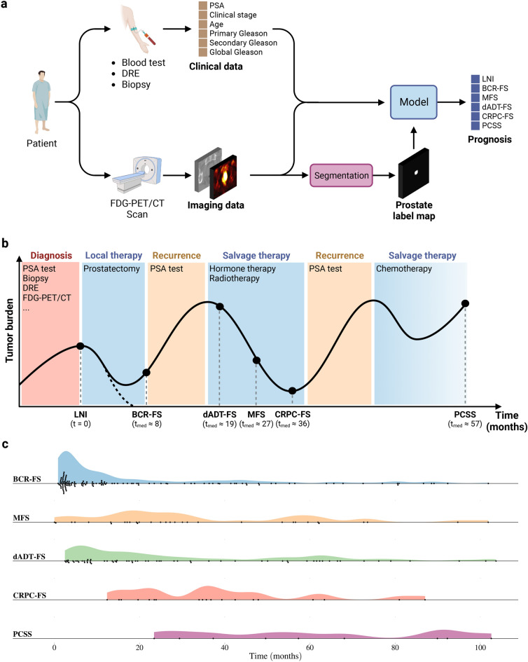
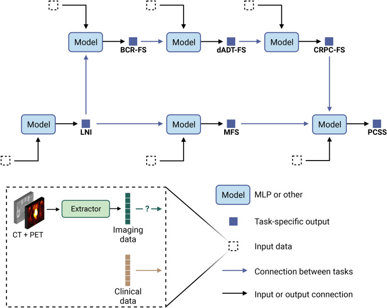
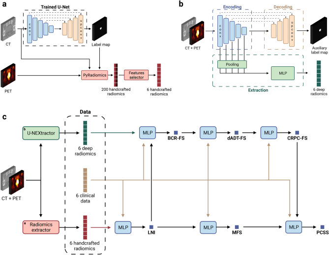
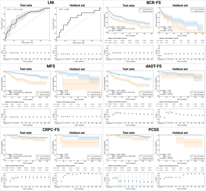
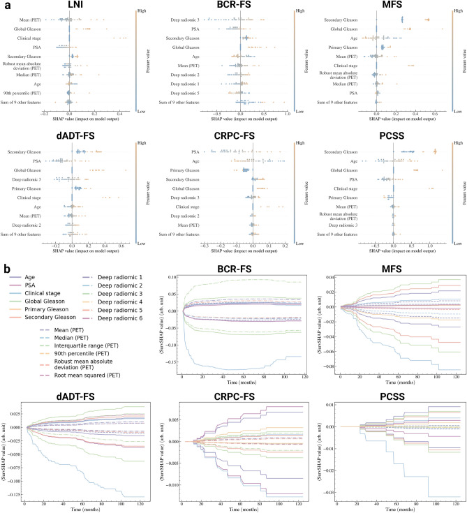
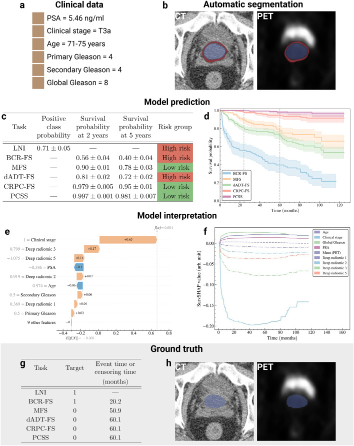
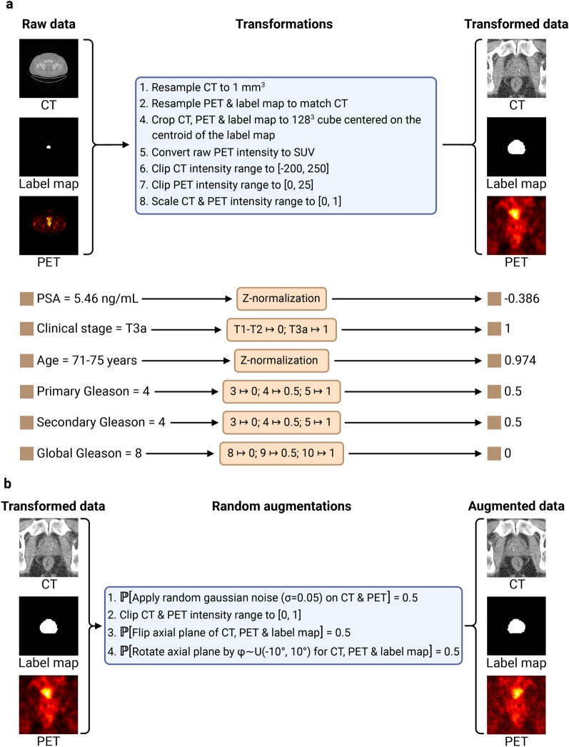
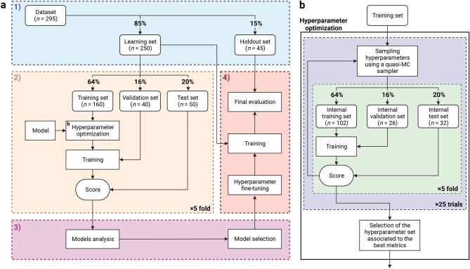
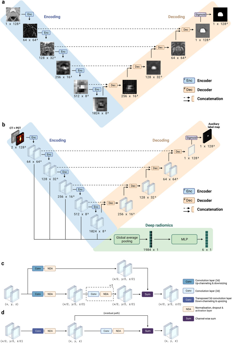
We propose a fully automatic multi-task Bayesian model, named Bayesian Sequential Network (BSN), for predicting high-grade (Gleason $\ge$ 8) prostate cancer (PCa) prognosis using pre-prostatectomy FDG-PET/CT images and clinical data. BSN performs one classification task and five survival tasks: predicting lymph node invasion (LNI), biochemical recurrence-free survival (BCR-FS), metastasis-free survival, definitive androgen deprivation therapy-free survival, castration-resistant PCa-free survival, and PCa-specific survival (PCSS). Experiments are conducted using a dataset of 295 patients. BSN outperforms widely used nomograms on all tasks except PCSS, leveraging multi-task learning and imaging data. BSN also provides automated prostate segmentation, uncertainty quantification, personalized feature-based explanations, and introduces dynamic predictions, a novel approach that relies on short-term outcomes to refine long-term prognosis. Overall, BSN shows great promise in its ability to exploit imaging and clinicopathological data to predict poor outcome patients that need treatment intensification with loco-regional or systemic adjuvant therapy for high-risk PCa.

Keywords: Bayesian; FDG-PET/CT; Multi-modal; Multi-task; Prognosis; Prostate cancer; Segmentation.

Fig. 1

Study overview. (a) Schematic outline of a patient’s journey from diagnosis to prognosis. Following an FDG-PET/CT scan, a physician manually delineates the prostate on the CT image to create a segmentation map. This map is used to train the model and is not needed to infer the prognosis of a new patient, as the trained model automatically performs segmentation. Indeed, the study aims to develop a fully automatic prognostic model that takes as input both clinical and imaging data without requiring any manual steps. (b) Schematic representation of the natural history of high-grade PCa^,. All patients in the cohort underwent radical prostatectomy (RP), and therefore, event time is measured from the date of RP. Note that $t_{\text{med}}$ is the median survival time, calculated based on data from the 250 patients in the learning set. See Supplementary Tables 7 & 8 for in-depth analyses of survival and follow-up time distributions, respectively. (c) Distributions of survival time in the learning set. Each marker corresponds to a patient who suffered the corresponding event. Distributions are consistent with the natural progression of PCa. See Supplementary Figs. 2a, 5a, 8a, 11a & 14a for the Kaplan-Meier curves of each survival task on the learning set and Supplementary Fig. 18 for distributions of event indicators. Created in BioRender. Larose, M. (2024) https://BioRender.com/l83s945.

Fig. 2

Framework of the Sequential Network (SN). SN is a multi-task model comprised of several single-task models. Single-task models can be any feed-forward neural network, such as a multi-layer perceptron (MLP). The output of each single-task model represents either positive class probability for classification tasks or event risk for survival tasks. Each model has 3 different input types: clinical data (mandatory), imaging data (task-specific), and predictions from previous models (task-specific), hence the terminology “sequential”. The sequence of tasks was determined based on the natural history of prostate cancer (see Fig. 1b). See Supplementary Fig. 1 for the correlation between each pair of tasks. Created in BioRender. Larose, M. (2024) https://BioRender.com/g04v672.

Fig. 3

Sequential Network (SN). (a) Handcrafted radiomic features extraction pipeline. The U-Net, trained with manual contours, automatically generates a prostate segmentation map from the CT image (see Fig. 9a for the visualization of feature maps in different layers of the U-Net). A total of 200 radiomic features are computed with the pyradiomics Python library (see Supplementary Tables 21  & 22 for extraction parameters on CT and PET images, respectively), using voxels from both CT and PET images within the segmented region. The Gini importance of each feature is then determined using a random forest classifier with 10,000 trees implemented with the scikit-learn Python library and trained to predict a single task using 200 extracted radiomics. The 6 features with highest Gini importance are selected (see Supplementary Fig. 19 for selected features). (b) Deep radiomic features extraction pipeline. The model, named U-NEXtractor, segments the prostate and extracts deep radiomic features simultaneously. The idea is that the auxiliary segmentation task is expected to spatially guide the network to extract prognostically relevant features in the prostate region. See Fig. 9b for the U-NEXtractor’s detailed architecture. (c) Architecture of the final SN (see Fig. 2 for the conceptual framework). The input data for each single-task model is based on the data that yields the highest scores for MLP on the test sets. This refers to the best data (see Table 1, section B), i.e., clinical data and handcrafted radiomics for LNI, clinical data and deep radiomics for BCR-FS, and clinical data for MFS, dADT-FS, CRPC-FS, and PCSS. Created in BioRender. Larose, M. (2024) https://BioRender.com/e56u989.

Fig. 4

Visualization of the performance of selected models. Selected models are Bayesian Sequential Network (BSN) for all tasks except PCSS, which uses CAPRA score. For the classification task (i.e. LNI), receiver operating characteristic (ROC) curves on the test sets (top left) and holdout set (top right) are shown. The ROC curve on test sets corresponds to the mean (line) and standard deviation (shade) of the ROC curves on the 5 test sets. For each survival task, the model’s ability to stratify patients into clinically significant risk groups is illustrated by Kaplan-Meier curves of test sets (top left) and holdout set (top right) using stratification based on predicted risk (see Methods, section Risk groups, for a description of the risk threshold computation method). The 95% confidence interval (95% CI, shade) of the Kaplan-Meier curve (line) is estimated using log hazard. The p-value is computed using a log-rank test^,, which also provides statistics to calculate the hazard ratio (HR) and its 95% confidence interval. For each task, the performance of BSN’s dynamic predictions is shown both on test sets (bottom left) and holdout set (bottom right). Results show that dynamic predictions are refined over time as events unfold. Scores on the test sets correspond to the mean (marker) and standard deviation (error bar) of scores on the 5 test sets. Created in BioRender. Larose, M. (2024) https://BioRender.com/h69j095.

Fig. 5

Explanation of the predictions of selected models. Selected models correspond to the boxed models in Table 1, sections A, B & C, and predictions are made on the 45 patients in the holdout set. (a) SHapley Additive exPlanation (SHAP) values of every patient in the holdout set for each task. Features are ranked in order of mean absolute importance, with the most important at the top. For each feature, a marker is associated to each patient. (b) Time-dependent SHAP (SurvSHAP(t)) curves of the top 9 most important features shown in panel A for each survival task. For each Fig. 2 curves are shown per feature: one is the mean of strictly positive SurvSHAP(t) curves, and the other is the mean of strictly negative SurvSHAP(t) curves, both obtained from each patient in the holdout set. Created in BioRender. Larose, M. (2024) https://BioRender.com/n61c518.

Fig. 6

Illustration of a clinical application of selected models. The application involves establishing the prognosis of an arbitrarily selected patient from the holdout set. See Supplementary Figs. 20 & 21 for other examples of patient prognosis. (a) Patient’s clinical data. (b) Segmentation map of the prostate obtained from Bayesian U-Net trained on the learning set. The segmentation map is overlaid on CT and PET images to illustrate that the region of high FDG uptake by the bladder lies outside the segmentation map’s boundaries. The segmentation map is used to extract handcrafted radiomic features. Note that the DSC between automatic and manual segmentation (ground truth) is 0.910. Color code: average prostate segmentation map (blue) and standard deviation (red) over 100 inferences. See Supplementary Fig. 22a for the segmentation map obtained by Bayesian U-NEXtractor. (c) Average prediction and standard deviation of the model over 100 inferences. (d) Average survival curves predicted by the model (line) and 95% confidence interval (shade) over 100 inferences (e) Shapley additive explanation (SHAP) of the predicted risk of BCR-FS. (f) Time-dependent SHAP (SurvSHAP(t)) of the predicted risk of BCR-FS. (g) Ground truth progression of the patient’s cancer. Time represents the survival time when the target value is 1 and acts as a censoring time otherwise. (h) Ground truth prostate segmentation map obtained from manual contouring by a physician. Created in BioRender. Larose, M. (2024) https://BioRender.com/r08k904.

Fig. 7

Data preprocessing pipeline. (a) Data transformation pipeline. Following a 1 mm³ resampling of the CT image, the PET image and the manual prostate segmentation map (label map) are resampled to align with the voxels of the CT image. The position of the centroid of the label map, which corresponds to the centroid of the prostate, is computed and images are cropped to a 128 mm³ cube centered on this position. The PET volume is converted into standardized uptake value (SUV) image. The intensity of the CT and PET images are clipped to [− 200, 250] and [0, 25] respectively (see Methods, section Preprocessing for the clipping range selection methodology), and then mapped to [0, 1]. Continuous clinical features are standardized using z-normalization, while categorical features are mapped to numerical values using ordinal encoding. (b) Imaging data augmentation pipeline. After applying a small amount of random noise with 50% probability, the images are clipped to [0, 1] to ensure that the intensity of the transformed images remains in the same range as the untransformed images. Flipping and rotation are then applied with 50% probability. Created in BioRender. Larose, M. (2024) https://BioRender.com/r77u176.

Fig. 8

Experimental setup. (a) Overview of the model selection process. 1) Stratified division of the dataset into a learning set and a holdout set. See Supplementary Fig. 17  & 18 and Supplementary Tables 9 & 10 for visual and statistical comparison between the two generated sets. Stratification is based on LNI class labels and BCR-FS event indicators. 2) Evaluation of the models on 5 test sets using stratified 5-fold cross-validation. 3) Comparison and selection of the models based on performance and interpretability. The performance is measured using the mean and standard deviation of the scores on the 5 test sets. 4) Final evaluation of the selected model on the holdout set. (b) Detailed diagram of the Hyperparameter optimization box shown in section 2 of panel a. Hyperparameter optimization is performed automatically using the quasi-Monte Carlo (MC) sampler from the BoTorch Python library, which is used under the framework of the Optuna Python library. A total of 25 sets of hyperparameter values are sequentially sampled using the quasi-MC sampler and evaluated on the same 5 internal test sets. The performance is measured using the mean of the scores on the 5 internal test sets. The first 5 sets of hyperparameter values are randomly generated, while the subsequent ones are determined based on the performance score of the preceding sets. The set of hyperparameter values associated to the highest AUC (for classification tasks) or CI (for survival tasks) is selected. See Supplementary Tables 11–17 for hyperparameter search spaces and Supplementary Tables 18–20 for selected hyperparameter values. Created in BioRender. Larose, M. (2024) https://BioRender.com/n79f502.

Fig. 9

Architecture of the convolutional neural networks. (a) 3D U-Net with residual units. Size refers to channels $\times$ spatial dimensions. A grid pattern in the feature maps of the decoder appears due to padding in transposed convolution operations. See Supplementary Tables 11 & 20 for hyperparameters. (b) Architecture of the 3D U-NEXtractor with residual units. The model is trained to segment the prostate and extract deep radiomic features simultaneously. The segmentation task guides the extraction of prognostically significant features within the prostate region. See Supplementary Tables 11 & 19 for hyperparameters. (c) Encoder block. This block represents a function that reduces the size of each dimension of the input tensor by a factor of 2 using a strided convolution. (d) Decoder block. This block increases the size of each dimension of the input tensor by a factor of 2 using a strided transposed convolution. Created in BioRender. Larose, M. (2024) https://BioRender.com/a55p729.

References

1. Siegel, R. L., Giaquinto, A. N. & Jemal, A. Cancer statistics, 2024. CA A Cancer J. Clin.74, 12–49 (2024). - PubMed
1. Wilt, T. J. et al. Systematic review: Comparative effectiveness and harms of treatments for clinically localized prostate cancer. Ann. Intern. Med.148, 435–448 (2008). - PubMed
1. Jeffrey Albaugh, M. Measurement of quality of life in men with prostate cancer. Clin. J. Oncol. Nurs.12, 81 (2008). - PubMed
1. Sanda, M. G. et al. Quality of life and satisfaction with outcome among prostate-cancer survivors. N. Engl. J. Med.358, 1250–1261 (2008). - PubMed
1. Shariat, S. F., Karakiewicz, P. I., Suardi, N. & Kattan, M. W. Comparison of nomograms with other methods for predicting outcomes in prostate cancer: A critical analysis of the literature. Clin. Cancer Res.14, 4400–4407 (2008). - PubMed
Substances
LinkOut - more resources