A cellular basis for mapping behavioural structure

Abstract

To flexibly adapt to new situations, our brains must understand the regularities in the world, as well as those in our own patterns of behaviour. A wealth of findings is beginning to reveal the algorithms that we use to map the outside world^1-6. However, the biological algorithms that map the complex structured behaviours that we compose to reach our goals remain unknown. Here we reveal a neuronal implementation of an algorithm for mapping abstract behavioural structure and transferring it to new scenarios. We trained mice on many tasks that shared a common structure (organizing a sequence of goals) but differed in the specific goal locations. The mice discovered the underlying task structure, enabling zero-shot inferences on the first trial of new tasks. The activity of most neurons in the medial frontal cortex tiled progress to goal, akin to how place cells map physical space. These 'goal-progress cells' generalized, stretching and compressing their tiling to accommodate different goal distances. By contrast, progress along the overall sequence of goals was not encoded explicitly. Instead, a subset of goal-progress cells was further tuned such that individual neurons fired with a fixed task lag from a particular behavioural step. Together, these cells acted as task-structured memory buffers, implementing an algorithm that instantaneously encoded the entire sequence of future behavioural steps, and whose dynamics automatically computed the appropriate action at each step. These dynamics mirrored the abstract task structure both on-task and during offline sleep. Our findings suggest that schemata of complex behavioural structures can be generated by sculpting progress-to-goal tuning into task-structured buffers of individual behavioural steps.

Fig. 1. Mice learn an abstract task structure.

a, Task design. Mice learned to navigate between 4 sequential goals on a 3 × 3 spatial grid maze. Reward locations changed across tasks but the abstract structure, four rewards arranged in an ABCD loop, remained the same. A brief tone was played upon reward delivery in location a. b, When allowed to reach peak performance (70% shortest path transitions or 200 trial plateau), mice readily reached near-optimal performance in the last 20 trials, as demonstrated by comparing path length between goals to the shortest possible path (‘relative path distance’). Two-sided t-test against chance (6.44): n = 13 mice, t-statistic = −43.2, P = 1.54 × 10⁻¹⁴, d.f. = 12. c, Performance improved across the initial 20 trials of each new task. This improvement was markedly more rapid for the last five tasks compared to the first five tasks. A two-way repeated-measures ANOVA (n = 13 mice) showed a main effect of trial: F = 11.7, P = 1.5 × 10⁻⁵, d.f.₁ = 19, d.f.₂ = 228; task: F = 35.0, P = 7.1 × 10⁻⁵, d.f.₁ = 1, d.f.₂ = 12; and trial × task interaction: F = 2.99, P = 0.030, d.f.₁ = 19, d.f.₂ = 228. Lines in lighter shades represent performance of individual mice. d, Performance on the first trial improved markedly across tasks. One-way repeated measures ANOVA (n = 9 mice; only 9 of the 13 mice were presented with all 40 tasks) showed a main effect of task: F = 2.73, P = 0.016, d.f.₁ = 7, d.f.₂ = 42. Lines in lighter shades represent performance of individual mice (4 mice only completed 10 tasks). e, Mice readily performed zero-shot inference on the first trial of late tasks but not in early tasks. The proportion of tasks in which mice took the most direct path from d to a on the first trial is compared to premature returns from c to a and b to a. Two-sided Wilcoxon test; early tasks: n = 13 mice, W-statistic = 17.5, P = 0.168; late tasks: n = 13 mice, W-statistic = 3.0, P = 0.004. Data are mean ± s.e.m.

Fig. 2. Progress-to-goal is a key feature of task-tuned neurons in the medial frontal cortex.

a, 3D rendering of probe channel positions, with the inset showing mFC regions (Using HERBs). Contacts were mostly in prelimbic cortex (PrL) but also in anterior cingulate cortex (ACC), infralimbic cortex (IrL) and secondary motor cortex (M2). Mouse IDs: 0, me08; 1, ah03; 2, me10; 3, me11; 4, ah04; 5, ab03; 6, ah07. b, Schematics of polar plots used to project neuronal activity onto the circular task structure. The radial and angular axes represent firing rate and task position, respectively. Dashed lines along the cardinal directions represent reward (goal) times in each state. c, Neurons are tuned to the relative progress to goal of the mouse (goal-progress tuned). Top, a raster plot of firing activity in one state (C: orange segment of polar plot below) of a cell that consistently fires shortly before a goal is reached. Bottom, polar plots of task activity for five separate neurons, with maximum firing rates (Hz) on the top right of each polar plot. d, Bottom, some goal-progress-tuned cells are additionally modulated by state in a given task (goal-progress + state-tuned). Top, polar plots and spatial maps for a spatially tuned and state-tuned neuron (left) and a non-spatially tuned and state-tuned neuron (right) across two distinct task configurations. e, Two example goal-directed paths and overlaid spiking of three mFC neurons tuned to early, intermediate and late goal progress, regardless of the spatial trajectory of the mouse. f, Goal-progress tuning is consistent across tasks that differ in reward locations. Left, the average firing rate vector of all neurons relative to an individual goal (averaged across all states) arranged by peak goal-progress bin in task X. This alignment is largely maintained in tasks Y and Z as well as a later session of the first task (X′). Right, histogram showing the mean goal-progress vector correlation across tasks for each neuron. One-sample, two-sided t-test against 0: n = 2,461 neurons; t-statistic = 104.3; P = 0.0, d.f. = 2,460. g, Pie chart showing the proportion of all neurons that are goal-progress tuned: 74%; two proportions test: n = 1,252 neurons, z = 35.5, P = 0.0. h, Plot of the mean task manifold derived from UMAP embedding. The same manifold is shown twice to emphasize goal-progress tuning (left) and state tuning (right). The task manifold is composed of goal-progress subloops. i, Distances along the three-dimensional manifold across different states and opposite goal-progress bin, across different states but for the same goal-progress bin or across different states and same goal-progress bin for a shuffled control. n = 20 double days; two-sided t-tests with Bonferroni correction: across-goal progress versus within-goal progress: t-statistic = 6.09, P = 2.25 × 10⁻⁵, d.f. = 19; across-goal progress versus permuted control: t-statistic = 26.0, P = 7.85 × 10⁻¹⁶, d.f. = 19; within-goal progress versus permuted control: t-statistic = 8.63, P = 1.60 × 10⁻⁷, d.f. = 19. Data are mean ± s.e.m. a.u., arbitrary units.

Fig. 3. Medial frontal neurons are organized into task-space modules.

a, Simultaneously recorded neurons readily remap their state tuning but maintain their goal-progress preference across tasks. Angles (in degrees) of each cell’s rotation relative to session X are shown on the right of each polar plot. b, Top, schematic showing quantification of tuning angle across sessions. Bottom left, polar histograms of cross-task angle show no single neuron generalization across tasks, with no clear peak at zero relative to the other cardinal directions (two proportions test against a chance level of 25%; n = 1,594 neurons; mean proportion of generalizing neurons across one comparison (mean of X versus Y and X versus Z) = 24%, z = 0.91, P = 0.363. Bottom right, neurons maintain their state preference across different sessions of the same task (X versus X′, two proportions test against a chance level of 25%; n = 1,160 neurons; proportion generalizing = 78%, z = 25.7, P = 0.0). c, Top, schematic showing quantification of relative angle difference between pairs of neurons across sessions. Bottom left, polar histograms show that the proportion of coherent pairs of state-tuned neurons (comprising the peak at zero) is higher than chance but less than 100%, indicating that the whole population does not remap coherently. Two-proportions test against a chance level of 25%; n = 35,164 pairs; mean proportion of coherent neurons across one comparison (mean of X versus Y and X versus Z) = 29.3%, z = 13.0, P = 0.0). Bottom right, as expected from b, the large majority of state-tuned neurons keep their relative angles across sessions of the same task (X versus X′; two proportions test against a chance level of 25%; n = 23,674 pairs; proportion coherent = 63%, z = 83.5, P = 0.0). d, Left, example from a single recording day showing the result of t-distributed stochastic neighbour embedding and hierarchical clustering derived from a distance matrix quantifying cross-task coherence relationships between state-tuned neurons. Each dot represents a neuron. Right, summary silhouette scores for the clustering for real data compared to permuted data that maintains the neuron’s goal-progress preference and initial state distribution. Each dot is a recording day. Two-sided Wilcoxon test: n = 38 recording days; W-statistic = 126.0, P = 2.13 × 10⁻⁴. e, Modules in a single recording day. The colour code represents the tuning of the neurons in task X. The x,y position defines the tuning in each task. The z position corresponds to (arbitrary) cluster IDs. Neurons remap in task space while maintaining their within-cluster but not between-cluster tuning relationships across tasks.

Fig. 4. The structured memory buffers model.

a, A hypothetical task-structured memory buffer (SMB) in the ABCD task. This ring-shaped SMB is a buffer for a specific behavioural step (goal in location 1): neurons along the SMB represent task position relative to this behavioural step. This behavioural step is therefore the anchor for this SMB. Aligning neurons by when a rewarded goal is encountered in location 1 reveals the invariant relationships between neurons across any two tasks where location 1 is rewarded. The dark blue anchor neuron (neuron 1) responds directly to goal location 1. Conversely, 3 other neurons fire at lags of 90° (one state away), 180° and 270° from the anchor. Other neurons (white circles) encode lags that are not necessarily multiples of 90°. The SMB is shaped by the task, which in the ABCD loop task means that activity circles back to the anchor point after four rewarded goals. b, Two example ABCD tasks that share one goal location (location 1, marked by X). Shaded regions show the spatial firing fields of each of the four neurons shown in a. Whereas the anchor neuron (neuron 1; dark blue) fires consistently at goal location 1 across tasks, other neurons (neurons 2–4; lighter shades of blue) fire in different locations in the two tasks. This spatial remapping is not random, but rather preserves encoding of elapsed task progress from goal in location 1. c, The same ring as in a, when aligned by the abstract task states (for example, state A), appears to rotate by 180° across tasks. This is because location 1 is rewarded in different states across tasks (state A in task 1 and state C in task 2). All neurons on the SMB remap by the same amount, not just the spatially tuned anchor neuron. d, A time series showing the flow of activity along 4 SMBs, each anchored to one of the 4 rewarded locations in task 1. A bump of activity is initiated in each SMB when its anchor is visited (top) and moves along the SMB paced by the progress of the mouse in task space. When it circles back close to the start, it biases the mouse to return to the behavioural step encoded by the anchor of the SMB. Multiple SMBs have active bumps at any one time, thereby simultaneously tracking a sequence of behavioural steps for an entire trial. In principle, the same computational logic can also be used even when individual neurons respond to more than one anchor and/or lag. The readout in such a scenario would involve combinatorial activity across anchor neurons from multiple SMBs. Reproduced/adapted with permission from Gil Costa.

Fig. 5. Medial frontal neurons track task progress from specific behavioural steps.

a, Single anchor alignment analysis. Top plot (blue) shows activity aligned by the abstract states; state tuning remaps across tasks. Bottom plot (green) shows the same neuron aligned to the behavioural step (goal-progress/location conjunction) to which it is anchored (dashed vertical line). In this and the other analyses in this figure, we concatenated two recording days, giving a total of up to six new tasks per neuron. b, Polar histograms showing the cross-validated alignment of neurons by their preferred anchor (calculated from training tasks) in a left-out test task. The top plot is for all state-tuned neurons, whereas the bottom plot only includes non-zero lag neurons. Two-proportions test against chance (25%), proportion generalizing for all state-tuned neurons: 39%, n = 738 neurons, z = 5.69, P = 1.24 × 10⁻⁸; non-zero lag state-tuned neurons: 36%, n = 545 neurons, z = 3.87, P = 1.08 × 10⁻⁴. c, Histograms showing the right-shifted distribution of the mean cross-validated task map correlations between state-tuned neurons aligned to their preferred anchor (from training tasks) and the task map aligned to this same anchor from a left-out test task. This is shown for all state-tuned neurons (top) and only non-zero lag state-tuned neurons (bottom). Two-sided t-test against 0 for all state-tuned neurons: n = 737 neurons, t-statistic = 9.86, P = 1.32 × 10⁻²¹, d.f. = 736; non-zero lag state-tuned neurons: n = 544 neurons, t-statistic = 7.55, P = 1.86 × 10⁻¹³, d.f. = 543. d, Two example paths of mice during a trial in two distinct tasks with two simultaneously recorded mFC neurons. Neuron 1 is an anchor neuron tuned to reward in location 6. Neuron 2 fires with a lag of roughly 270° in task space from its anchor (reward in location 6). Spikes are jittered to ensure directly overlapping spikes are distinguishable. e, Lagged spatial field analysis. Bottom, each row represents a different task and each column represents a different lag in task space, starting from the current location of the mouse (far right column) and then at successive task space lags in the past or future. Because of the circular nature of the task, past bins at lag X are equivalent to future bins at lag 360 - X. Right, zoomed in spatial maps at this neuron’s preferred lag. Top, the correlation of spatial maps across tasks at each lag. Colours are normalized per map to emphasize the spatial firing pattern, with maximum firing rates (in Hz) displayed at the top right of each map. f, Histograms showing the right-shifted distribution of the mean cross-validated spatial correlations between maps at the preferred lag (from training tasks) and the spatial map at this lag from a left-out test task for all state-tuned neurons (left) and only non-zero lag neurons (right). Two-sided t-test against 0 for all state-tuned neurons: n = 738 neurons, t-statistic = 22.6, P = 1.45 × 10⁻⁸⁶, d.f. = 737; non-zero lag state-tuned neurons: n = 285 neurons, t-statistic = 7.48, P = 9.07 × 10⁻¹³, d.f. = 284. g, Left, regression analysis reveals neurons with lagged fields in task space from a given anchor (goal-progress/place conjunction). Right, this enables prediction of state tuning and its remapping across tasks for each neuron. h, Histograms showing the right-shifted distribution of mean cross-validated correlation values between model-predicted (from training tasks) and actual (from a left-out test task) activity. This correlation is shown for all state-tuned neurons (left) and only state-tuned neurons with non-zero-lag firing from their anchors (right). Two-sided t-test against 0 all state-tuned neurons (with non-zero beta coefficients): n = 489 neurons, t-statistic = 9.3, P = 5.3 × 10⁻¹⁹, d.f. = 488; non-zero lag state-tuned neurons: n = 329 neurons, t-statistic = 3.9, P = 1.08 × 10⁻⁴, d.f. = 328. Data are mean ± s.e.m.

Fig. 6. Medial frontal activity predicts distal behavioural choices.

a, Schematic showing distal prediction of choices from memory buffers. The SMB model enables us to predict the choices made by the mouse: (1) at a precise lag in the future; and (2) in a way that generalizes across tasks. The size and the timing of the activity bump determines how likely and when (respectively) the animal will visit the SMB’s anchor in the next trial. This future prediction should generalize across tasks and thus be independent of where the mouse is at a given time. In this example we show an SMB with an anchor at location 2 (top middle location shaded in brown) at intermediate goal progress (halfway between goals). The brown neuron is the anchor, whereas the green neuron fires at a lag of 1.5 states (135°) from the anchor. Four rows correspond to four possible scenarios across two different tasks, illustrating the key features of the SMB model’s predictions. The activity of the green neuron at precisely 1.5 states since the first anchor visit (t₂; the bump time of the green neuron) can be used to predict what will happen at t₃ (2.5 states forward from t₂). A larger activity bump (indicated by the height of the bump along the SMB) increases the likelihood that the animal will return to the anchor at t₃. This larger bump is indexed by higher activity of the green neuron at t₂ (indicated by a darker green shade). In task Y, the green neuron fires at a different location in order to keep its lag from its anchor. Nevertheless, its activity at t₂ can be used in the same way to predict whether the mouse will visit the anchor at t₃ (2.5 states in the future). To test this latter point, we only consider non-zero lag cells, which fire in different locations across tasks, in all of the analyses below. Reproduced/adapted with permission from Gil Costa. b, Design of logistic regression to assess the effect of each neuron’s activity on future visits to its anchor. To control for autocorrelation in behavioural choices, previous choices as far back as ten trials in the past are added as co-regressors. Separate regressions are done for activity at different times: bump time, random times, decision time (the time where the mouse was one spatial step away, and one goal-progress bin away from the anchor of a given neuron) and times shifted by 90° intervals relative to the neuron’s bump time. c, Bottom, regression coefficients are significantly positive for the bump time but not for any of the other control times. Two-sided t-tests against 0 for bump time: n = 131 tasks, t-statistic = 2.75, P = 0.007, d.f. = 130; decision time: n = 131, t-statistic = −0.77, P = 0.446, d.f. = 130; random time: n = 131, t-statistic = −0.79, P = 0.433, d.f. = 130; 90° shifted time: n = 131, t-statistic = −2.74, P = 0.007, d.f. = 130; 180° shifted time: n = 131, t-statistic = −1.47, P = 0.143, d.f. = 130; 270° shifted time: n = 131, t-statistic = −2.54, P = 0.012, d.f. = 130. Top, swarm plots showing distribution of regression coefficient values across groups. Data are mean ± s.e.m.

Fig. 7. Offline activity of mFC neurons is internally organized by the task structure.

a, Schematic showing potential neuronal state spaces. Neuronal state space relationships are best described by circular distance for a ring and forward distance for a delay line. Reproduced/adapted with permission from Gil Costa. b, Schematic showing the linear regression model relating pairwise circular distance and forward distance with coactivity during sleep while regressing out each other, as well as pairwise goal-progress-tuning distance and spatial map similarity. c, Regression coefficient values for circular distance against sleep cross-correlation were more negative for pairs sharing the same anchor (within) compared with pairs across anchors (between). One-sided unpaired t-test (Welch’s t-test) for all sleep: n = 430 pairs (within), 13,932 pairs (between), t = −1.80, P = 0.036, d.f. = 14,360. d, A plot of sleep cross-correlations (between pairs sharing the same anchor) against forward and circular distance (bottom and top x axes, respectively). Schematics at the top and bottom show example pairs that would fall into each category and their circular and forward distances. The v-shaped relationship between forward distance and cross-correlation indicates a circular state space. Inset, kernel density estimate plots showing distribution of cross-correlation values across bins. Reproduced/adapted with permission from Gil Costa. e, Bar graph (top) and scatter plot (bottom) of correlation coefficients between pairwise forward distance and pairwise sleep cross-correlations are positive for pairs of neurons with 180–360° forward distance and negative for pairs with a forward distance of 0–180°. Two-sided t-tests relative to 0, 0–180°: n = 59 sleep sessions, t-statistic = −5.16, P = 1.07 × 10⁻⁴, d.f. = 58; 180–360°: n = 59 sleep sessions, t-statistic = 4.16, P = 1.08 × 10⁻⁴, d.f. = 58. Two-sided paired t-test: n = 59 sleep sessions, t-statistic = −5.55, P = 7.35 × 10⁻⁷, d.f. = 58. Data are mean ± s.e.m. In c, this error is analytically derived for each regression; thus there are no individual points to report in this panel.

Extended Data Fig. 1. Behavioural measures in the ABCD task.

a) Three example connection configurations for the pre-selection and pre-training sessions done before exposure to the first ABCD task. Here a subset of 5-7 maze locations (nodes) were available to the mouse and each node was rewarded provided the animal did not just receive reward in the same node. b) Tasks were designed such that task space and physical space are orthogonal to each other. Left: schematic showing that optimal path lengths between rewarded goals differed both within and between tasks. Right: a bar plot showing that the task space “distances” between reward locations (how many task states are between the rewards) are not correlated with the physical distances in the maze (the optimal number of steps taken to reach reward). Data points represent individual mice, where physical distances are averaged across all tasks experienced by a given mouse. Pearson correlation: r = 6.04 × 10-18 P = 1.0; one-way ANOVA statistic=2.02, P = 0.147, df = 12 c). Example paths from 3 different mice performing 3 different tasks. Each row is a set of 5 consecutive trials from the same mouse and task. Single trial paths are superimposed upon whole session coverage shown in grey. Mice rapidly converged on near-optimal routes and used only a subset of the available paths. d) Reward sequences showed minimal correlation across all tasks in all mice (left) and no correlations on all tasks for mice where neuronal data was recorded (7/13 mice middle) or on the late 3 task days from neural mice (right). Note that electrophysiological data in this manuscript is all collected from the late 3 task days. T-test (two-sided) against 0 correlation: all tasks: N = 13 mice, r = 0.002, statistic=2.91, P = 0.013, df = 12; all tasks from neural mice (mice where neuronal data was recorded): N = 7 mice, r = 0.002, statistic=1.81, P = 0.120, df = 6; tasks on Late 3-task days from neural mice (tasks where neural data was recorded): N = 7 mice, r = 4.5 × 10⁻⁴, statistic=0.22, P = 0.634, df = 6. e) Animals used stereotyped routes when taking the shortest route to a goal. The entropy of correct transitions taken is lower than expected if animals took all shortest routes equally. T-test (two-sided) against 1 – N = 13 animals, statistic = −23.6, P = 1.96 × 10⁻¹¹, df = 12 f) Performance is unaffected by the inclusion of a tone at reward a. 3 mice were exposed to additional tasks (after completing task 40) where the tone at a was randomly omitted in 50% of trials. The tone or no-tone status of a trial refers to whether the tone was omitted at the a at the beginning of the trial. Left: mean proportion of transitions where one of the shortest routes was taken N = 26 tasks, Wilcoxon test (two-sided); statistic=164, P = 0.784. Right: mean relative path distance N = 26 tasks, Wilcoxon test (two-sided): statistic=130, P = 0.258 g). Performance on the d-to-a transition is unaffected by the inclusion of a tone at reward a in the previous trial: Left: mean proportion of transitions where one of the shortest routes was taken N = 26 tasks, Wilcoxon test (two-sided); statistic=134, P = 0.903. Right: mean relative path distance N = 26 tasks, Wilcoxon test (two-sided): statistic=149, P = 0.515 h). Suboptimal performance was associated with persisting behavioural biases from before exposure to the task. Y-axis shows the r value calculated from a correlation between the mean relative path distance taken between goals and the probability the steps within this trajectory would have been taken when the animal was naive to any ABCD task (when the animal explored the arena before any rewards or tasks were presented). A net positive correlation indicates that when animals take longer routes (i.e. perform less optimally) they take these routes through steps that they were more likely to take before exposure to any ABCD task. T-test (two-sided) against 0 – N = 13 animals, statistic=2.70, P = 0.019, df = 12 i). Mean relative path distance travelled by the mice between goals in the first 20 trials of early vs late tasks. Wilcoxon test (two-sided) N = 13 animals, Statistic=0.0, P = 2.44 × 10⁻⁴ j). Mean proportion of transitions where one of the shortest routes was taken in the first 20 trials of early vs late tasks. Wilcoxon test (two-sided) N = 13 animals, Statistic=10.0 P = 0.010 k) Mean proportion of “perfect trials” where all transitions (a → b, b → c, c → d and d → a) in a given trial were taken via the shortest route. Left: scatter plot of mean proportion of perfect trials in the first 20 trials of early vs late tasks. Wilcoxon test (two-sided) N = 13 animals, Statistic=11.0 P = 0.028. Right: bar plot of the same data showing that, for both early and late tasks, the proportion of perfect trials is significantly above chance: T-test (two-tailed) against chance (0.007): Early tasks statistic=2.55, P = 0.025; Late tasks - statistic=4.06, P = 0.002. l) ABCDE task performance (relative path distance): after completing at least 40 ABCD tasks, two animals completed additional ABCDE tasks (11 and 13 tasks each) where tasks comprised a loop of 5 (instead of 4) rewards. Animals readily performed above chance in the first 20 trials, as demonstrated by comparing path length between goals to the shortest possible path (i.e. computing a “relative path distance” measure). T-test (two-sided) against chance (6.44): N = 24 tasks, statistic = −30.0 P = 6.18 × 10⁻²⁰, df = 23. Chance level was calculated empirically using the mean relative path distance across the first trial of the first 5 ABCD tasks. m) ABCDE task performance (proportion correct transitions): animals readily performed above chance in the first 20 trials, as demonstrated by quantifying the proportion of transitions where animals took the shortest possible path. Wilcoxon test (two-sided): N = 24 tasks, statistic=0.0, P = 1.19 × 10⁻⁷. Chance levels were derived empirically for each mouse using baseline transition probabilities calculated when animals explored the maze before experiencing any ABCD tasks: see Methods under “Behavioural Scoring”. n) No difference in the empirical chance levels (baseline transition probabilities calculated when animals explored the maze before experiencing any ABCD tasks: see Methods under “Behavioural Scoring”) between d-to-a and c-to-a/b-to-a transitions on the first trial in early (left) and late (right) tasks. Wilcoxon test (two-sided); Early tasks: N = 13 animals, statistic=42.0, P = 0.839; Late tasks: N = 13 animals, statistic=43.0, P = 0.893 o). No difference in the analytical chance levels (see Methods under “Behavioural Scoring”) between d to a and c-to-a/b-to-a transitions on the first trial in early (left) and late (right) tasks. Wilcoxon test (two-sided); Early tasks: N = 13 animals, statistic=20.0, P = 0.080; Late tasks: N = 13 animals, statistic=32.0, P = 0.376 p). No difference in the shortest physical maze distances between d-to-a and c-to-a/b-to-a transitions on the first trial in early (left) and late (right) tasks. Wilcoxon test (two-sided); Early tasks: N = 13 animals, statistic=16.0, P = 0.071; Late Tasks: N = 13 animals, statistic=25.0, P = 0.477 q) Zero-shot inference on the first trial of late tasks is associated with animals returning from d to a more often than d-to-b or d-to-c. The proportion of tasks in which animals took the most direct path from d-to-a on the first trial is compared to the same measure but for premature returns from d-to-b and d-to-c. Early tasks are shown on the left and late tasks on the right. Wilcoxon test (two-sided); Early tasks: N = 13 animals, statistic=27.0, P = 0.594; N = 13 animals, Late tasks: statistic=6.0, P = 0.016 All error bars represent the standard error of the mean.

Extended Data Fig. 2. Recording set up and tuning properties of mFC neurons in the ABCD task.

a) Coronal slice from an implanted mouse showing silicon probe track terminating in the prelimbic region of mFC. b) The laminar profile of probe channel positions for each mouse. Shanks A-F in Cambridge neurotech probes are arranged posterior-to-anterior. 90.7% of all recorded neurons were histologically localised in mFC regions based on the inferred channel position: 68.3% in Prelimbic cortex, 11.3% in Anterior Cingulate cortex, 6.1% in Infralimbic cortex and 5.0% in M2. Of the remaining 9.3%, 4.8% could not be localised to a specific peri-mFC region within the atlas coordinates as they were erroneously designated to peri-mFC white matter areas, likely due to variations between actual region boundaries and atlas derived ones, 2.2% were found in the dorsal peduncular nucleus, 1.1% in the striatum, 0.6% in the medial orbital cortex, 0.3% in the lateral septal nucleus and 0.3% in Olfactory cortex. c) Data was spike sorted across concatenated sessions spanning two recording days for the GLM analyses below and later anchoring analysis in Figs. 5–7. Top: Here we show an example “Estimated drift trace” for a concatenated double day, showing a largely stable recording set up. The plot shows the estimated probe drift relative to the brain across the two recording days along the depth of the neuropixels probe. Bottom: Example mean spike waveforms from 3 different neurons across 3 different animals. The plots show the mean of the first 100 spikes on day1 (black) and the mean of the last 100 spikes on day2 (red), illustrating stability of spike detection across days. The spikes are from neuron 1 and neuron 2 in Extended Data Fig. 6b and the neuron in Fig. 5e respectively. Scale bars: Vertical: 200 µV, Horizontal: 0.5 ms. d) Top: a schematic of the variables inputted into a generalised linear model that predicts neuronal activity across tasks and states. The model captured variance as a function of goal-progress, place, speed, acceleration, time from reward and distance from reward. Only data spike sorted across two days (6 unique tasks) was used to ensure this analysis is sufficiently powered. Bottom Left: A histogram showing the mean regression coefficient values for goal-progress as a regressor across task/state combinations for each neuron. One-sample T-test (two-sided) against 0: N = 1252 neurons; statistic=21.7; P = 8.93 × 10-89, df = 1251. Bottom right: A histogram showing the mean regression coefficient values for place as a regressor across task/state combinations for each neuron. One-sample T-test (two-sided) against 0: N = 1252 neurons; statistic=24.9; P = 3.31 × 10-111, df = 1251. e) Pie-charts showing the proportions of cells calculated using the results of the generalised linear model above in addition to cross-task correlations between tuning to goal-progress and place. Only data spike sorted across two days (6 unique tasks) was used to ensure this analysis is sufficiently powered. Plot shows proportions of neurons with i) significant regression coefficient values for goal-progress or place ii) Significantly positive cross-task correlation for goal-progress or place. It also shows proportions of state tuned neurons derived from a separate z-scoring analysis (More details in Methods under “Tuning to basic task variables”). Proportion of all neurons that are goal-progress cells: 74%; Two proportions test: N = 1252 neurons, z = 35.5, P = 0.0. Proportion of goal-progress neurons that are state tuned: 64% Two proportions test: N = 931 neurons, z = 26.8, P = 0.0. Proportion of neurons tuned to goal-progress and state that are also tuned to place: 63%, Two proportions test: N = 597 neurons, z = 21.2, P = 0.0. Proportion of all state-tuned neurons that are also goal-progress tuned; 81% Two proportions test: N = 738 neurons, z = 29.5, P = 0.0. f) A histogram showing the distribution of significant goal-progress peaks amongst all neurons, all tasks and all states. Only neurons from concatenated double days that are significantly goal progress-tuned and have at least one significant goal-progress peak are shown (N = 873 neurons). The plot shows that such significantly goal-progress tuned cells have peaks throughout the entire range of goal progress values. Note that this plot spans goal-progress space, which is the lag between any two rewarded goals, rather than the full (multi-goal) task space. g) Regression coefficients for animal kinematics (from GLM in Fig. 2g). Two histograms showing the mean regression coefficient values for Speed (Left) and Acceleration (Right) as a regressor across task/state combinations for each neuron. One-sample T-test (two-sided) against 0: Speed: N = 1252 neurons, statistic=3.36, P = 8.01 × 10⁻⁴ df = 1251; Acceleration: N = 1252 neurons, statistic = −0.78, P = 0.438 df = 1251. h) Polar plots of task tuning and spatial maps for four example neurons that are tuned to both goal-progress and state. Each neuron is plotted across two tasks to illustrate spatial tuning (left two neurons) and lack thereof (right two neurons). i) The subregional distribution of neuron type coefficients along the medial wall of the frontal cortex in neuropixels recordings. One-way ANOVA: Left: Proportion of Goal progress neurons: F = 2.40, P = 0.143, df = 3; Middle: Proportion of state neurons F = 1.04, P = 0.425, dof=3; Right: Proportion of place-tuned neurons F = 18.8, P = 5.54 × 10⁻⁴, df = 3. Posthoc Tukey HSD tests (Two-tailed): IrL vs PrL P = 0.049; IrL vs ACC P = 0.000; IrL vs M2 statistic=0.003, PrL vs ACC P = 0.021. j) A plot of the mean task manifold derived from a Uniform Manifold Approximation and Projection (UMAP)-embedding along three dimensions restricted to only non-spatial neurons. Note that we use the most permissive threshold for spatial tuning here to ensure that we exclude even neurons with weak/residual spatial tuning. Any neuron that had a spatial regression coefficient above the 95th percentile of the null distribution was excluded from this analysis. The same manifold is shown twice: Left, goal-progress tuning along the manifold; right, state tuning along the same manifold. The entire task manifold is composed of goal-progress subloops. k) Quantifications of distances along the 3-dimensional UMAP-derived manifold - across different states and opposite goal-progress bin (left), across different states but for the same goal-progress bin (middle) or the distances across different states and same goal-progress bin for a shuffled control. N = 8 double-days - T-tests (two-sided) (with bonferroni correction): Across-goal progress vs within goal-progress: statistic =10.3, P = 5.45 × 10⁻⁵, df = 7; Across-goal progress vs permuted control: statistic =17.5, P = 1.47 × 10⁻⁶, df = 7; Within goal-progress vs permuted control: statistic =5.2, P = 0.004, df = 7 All error bars represent the standard error of the mean.

Extended Data Fig. 3. Tuning properties of mFC neurons in the ABCDE task.

a) Polar plots of task-space tuning for 8 example neurons in the ABCDE task - neurons 1-4 are purely goal-progress tuned while neurons 5-8 are conjunctively goal-progress and state tuned. b) State neurons in the ABCDE task are predominantly goal progress tuned. Left: design of GLM to identify goal-progress tuned neurons in ABCDE tasks. Right pie chart showing the proportion of state-tuned neurons that are goal-progress tuned: ABCDE goal-progress/state GLM; Two proportions test: N = 189 state neurons, proportion goal-progress-tuned= 85%, z = 15.6, P = 0.0) c) Polar plots of task-space tuning for 3 example neurons recorded across 2 ABCD tasks and then two ABCDE tasks - neurons 1 is purely goal-progress tuned while neurons 2 and 3 are conjunctively goal-progress and state tuned. d) Goal progress tuning is maintained across abstract tasks ABCDE vs ABCD: The average firing rate vector of all neurons relative to an individual goal (from goal “n” to goal “n + 1”; averaged across all states). Animals experienced 2 ABCD tasks followed by 2 ABCDE tasks on these days. Each row represents a single neuron and the neurons are arranged on the y axis by their peak firing goal-progress in task 1 in the ABCD condition. This alignment is largely maintained in tasks across both ABCD and ABCDE structures. White dashes indicate early intermediate and late goal-progress-cutoffs. e) A histogram showing the mean goal-progress-vector correlation across tasks for each neuron. One-sample T-test (two-sided) against 0: N = 111 neurons; statistic=23.8; P = 3.76 × 10⁻⁴⁵, df = 110. Note that the neurons used in this panel are those on days where animals experienced both ABCDE and ABCD tasks. f) Left: design of GLM to identify whether neurons maintain their goal-progress tuning across ABCDE and ABCD tasks. Right: A histogram showing the mean regression coefficient values for goal-progress as a regressor across ABCD and ABCDE tasks for each neuron. One-sample T-test (two-sided) against 0: N = 111 neurons; statistic=7.43; P = 2.45 × 10⁻¹¹, df = 110. g) A plot of the mean task manifold derived from a Uniform Manifold Approximation and Projection (UMAP)-embedding along three dimensions for mFC activity in the ABCDE. The same manifold is shown twice: Left, goal-progress tuning along the manifold; right, state tuning along the same manifold. The entire task manifold is composed of goal-progress subloops. h) Quantifications of distances along the 3-dimensional UMAP-derived manifold - across different states and opposite goal-progress bin (left), across different states but for the same goal-progress bin (middle) or the distances across different states and same goal-progress bin for a permuted control. N = 4 double-days - T-tests (two-sided) (with bonferroni correction): Across-goal progress vs within goal-progress: statistic =6.64, P = 0.021, df = 3; Across-goal progress vs permuted control: statistic =21.1, P = 7.02 × 10⁻⁴, df = 3; Within goal-progress vs permuted control: statistic =10.7, P = 0.005, df = 3 All error bars represent the standard error of the mean.

Extended Data Fig. 4. Quasi-coherent task-space remapping of mFC neurons.

a) Three example state-tuned neurons remapping across tasks. The top two neurons remap in a way that is not related to their spatial maps in any given task. The bottom neuron remaps in accordance to its spatial map. Angles (in degrees) of each cell’s rotation relative to its tuning in session X are shown to the right of each session’s polar plot. Note that these are not all simultaneously recorded neurons. b) Remapping of state neurons that are defined using a stricter threshold (z-score >99th percentile of permuted distribution). Top: A schematic showing how the difference in tuning angles for the same neuron across sessions is quantified. Bottom left: Polar histograms show that state-tuned neurons remap by angles close to multiples of 90 degrees, as a result of conserved goal-progress tuning and the 4 reward structure of the task. No clear peak at zero is seen relative to the other cardinal directions when comparing sessions spanning separate tasks (Two proportions test against a chance level of 25% N = 1061 neurons; mean proportion of generalising neurons across one comparison (mean of X vs Y and X vs Z) = 24%, z = 0.59, P = 0.552. Bottom right: Neurons maintain their state preference across different sessions of the same task (X vs X’ Two proportions test against a chance level of 25% N = 770 neurons; proportion generalising=80%, z = 21.5, P = 0.0). c) Remapping when using only state-neurons with concordant remapping angles across two methods (i.e. using the best-rotation analysis method and peak-to-peak changes method). This analysis would for example exclude neuron 3 in Fig. 3a. Left: Polar histograms show that state-tuned neurons remap by angles close to multiples 90 degrees, as a result of conserved goal-progress tuning and the 4 reward structure of the task. No clear peak at zero is seen relative to the other cardinal directions when comparing sessions spanning separate tasks (Two proportions test against a chance level of 25% N = 369 neurons; mean proportion of generalising neurons across one comparison (mean of X vs Y and X vs Z) = 24%, z = 0.41 P = 0.684. Right: state-tuned neurons maintain their state preference across different sessions of the same task (bottom right). Two proportions test against a chance level of 25% N = 240 neurons; proportion generalising=84%, z = 13.0, P = 0.0). d) Remapping of non-spatial neurons. Note that we use the most permissive threshold for spatial tuning here to ensure that we exclude even neurons with weak/residual spatial tuning. Any neuron that had a spatial regression coefficient above the 95th percentile of the null distribution was excluded from this analysis. Left: Polar histograms show that non-spatial state-tuned neurons remap by angles close to multiples 90 degrees, as a result of conserved goal-progress tuning and the 4 reward structure of the task. No clear peak at zero is seen relative to the other cardinal directions when comparing sessions spanning separate tasks (Two proportions test against a chance level of 25% N = 704 neurons; mean proportion of generalising neurons across one comparison (mean of X vs Y and X vs Z) = 22%, z = 1.19 P = 0.233). Right: Non-spatial state-tuned neurons maintain their state preference across different sessions of the same task (bottom right). Two proportions test against a chance level of 25% N = 507 neurons; proportion generalising=68%, z = 13.9, P = 0.0). e) Pairwise coherence of state neurons that are defined using a stricter threshold (z-score >99th percentile of permuted distribution). Top: A schematic showing how the difference in relative angles between pairs of neurons across sessions is quantified. Bottom left: Polar histograms show that the proportion of coherent pairs of state-tuned neurons (comprising the peak at zero) is higher than chance but less than 100%, indicating that the whole population does not rotate coherently. Two proportions test against a chance level of 25% N = 17671 pairs; mean proportion of coherent neurons across one comparison (mean of X vs Y and X vs Z) = 29%, z = 8.9, P = 0.0). Bottom right: As expected from panel b, the large majority of state-tuned neurons keep their relative angles across sessions of the same task (X vs X’; Two proportions test against a chance level of 25% N = 11716 pairs; proportion coherent=64%, z = 59.3, P = 0.0). f) Coherence of state-neuron pairs using only state-neurons with concordant remapping angles across two methods (i.e. using the best-rotation analysis method and peak-to-peak changes method). Left: Polar histograms show that the proportion of coherent pairs of state-tuned neurons (comprising the peak at zero) is higher than chance but far from 1, indicating that the whole population does not rotate coherently (Two proportions test against a chance level of 25% N = 1642 pairs; mean proportion of coherent neurons across one comparison (mean of X vs Y and X vs Z = 30%, z = 3.32, P = 9.04 × 10⁻⁴). Right: As expected from panel b, the large majority of state-tuned neurons keep their relative angles across sessions of the same task (X vs X’; Two proportions test against a chance level of 25% N = 657 pairs; proportion coherent=72%, z = 17.1, P = 0.0). g) Coherence of non-spatial neuron pairs. Note that we use the most permissive threshold for spatial tuning here to ensure that we exclude even neurons with weak/residual spatial tuning. Any neuron that had a spatial regression coefficient above the 95th percentile of the null distribution was excluded from this analysis. Left: Polar histograms show that the proportion of coherent pairs of non-spatial state-tuned neurons (comprising the peak at zero) is higher than chance but far from 1, indicating that the whole population does not rotate coherently (Two proportions test against a chance level of 25% N = 6996 pairs; mean proportion of coherent neurons across one comparison (mean of X vs Y and X vs Z = 30%, z = 3.49, P = 4.74 × 10⁻⁴). Right: As expected from panel b, the large majority of non-spatial state-tuned neurons keep their relative angles across sessions of the same task (X vs X’; Two proportions test against a chance level of 25% N = 4822 pairs; proportion coherent=54%, z = 29.2, P = 0.0). h) Proportion of coherent pairs per recording day (pairs of state-tuned neurons where the relative angle doesn’t change by more than 45 degrees across both X to Y and X to Z comparisons) relative to all pairs across different pairwise task space angles. T-tests (two-sided) with Bonferroni correction against chance level of 1/16 (probability of neuron pair rotating coherently across two comparisons (i.e. 1/4²)): N = 38 recording days, pairwise circular distance difference: 0-45 degrees statistic=8.17, P = 3.33 × 10⁻⁹, df = 37; 45-90 degrees statistic=2.84, P = 0.013, df = 37; 90-135 degrees statistic=3.88, P = 0.001, df = 37; 135-180 degrees statistic=2.89, P = 0.013, df = 37. Top: bar graph, bottom: individual points (recording days). i) Coherent pairs are slightly closer anatomically than incoherent pairs. Mann-Whitney U-test (Two-sided): N = 3567 pairs (53 coherent; 3514 incoherent), statistic=72872, P = 0.006. Note that, to minimise the effect of noise, this analysis uses only double days and only considers a pair of neurons coherent if they show perfect coherence across all combinations of 6 tasks. Top: bar graph, bottom: kernel density estimate of data distribution. j) The subregional distribution of single neuron generalisation (averaged across X vs Y and X vs Z comparisons) along the medial wall of frontal cortex in neuropixels recordings. One-way ANOVA: F = 1.59, P = 0.323, df = 3. k) The subregional distribution of neuron pair coherence. Coherence is calculated across both X vs Y and X vs Z comparisons along the medial wall of frontal cortex in neuropixels recordings: One-way ANOVA: F = 4.76, P = 0.083, df = 3. l) Top: Visualisation of tuning relationships between two clusters computed in a single recording day. Each dot is a neuron (numbered in correspondence to the polar plots below) and each ring is a cluster derived from the analysis in panel d. The colour code represents the tuning of the neurons in task X. The x,y position defines the tuning in each task. The z position corresponds to cluster ID. Note that the ordering along the z axis is arbitrary. Neurons rotate (remap) in task space while maintaining their within-cluster tuning relationships but not cross-cluster relationships across tasks. Bottom: polar plots for all of the (seven) neurons assigned to each of the two clusters in the above plot. Angles (in degrees) of each cell’s rotation relative to its tuning in session X are shown to the right of each session’s polar plot. All error bars represent the standard error of the mean.

Extended Data Fig. 5. The Structured Memory buffers model predicts behavioural sequences.

a) As well as rings tracking task-progress from behavioural steps involving a rewarded place (a conjunction of a place with early goal-progress), there are also rings tracking task-progress from places conjoined with intermediate and late goal-progress. The anchors of these rings are activated when the animal passes through a location, not when it is rewarded, but at a defined, non-zero progress percentage relative to the upcoming goal. b) Non-zero goal-progress anchored rings (e.g. purple outline) allow tracking task-progress from behavioural steps in between two goals. Hence, across all rings, a history of the entire sequence of steps taken by the animal, not just the sequence of reward locations, is encoded at any one point in time. c) Schematic showing distal prediction of an animal’s choices from memory buffers. When the animal visits a goal-progress/place (t = 1) in trial N, a bump of activity is initiated in the memory buffer that is anchored to this goal-progress/place. The anchor is location 2 at intermediate goal progress (brown) in the top memory buffer, and location 4 at intermediate goal progress (red) in the bottom memory buffer. This bump travels around the buffer (e.g. t = 2), paced by progress in the task. When the activity bump circles back to a point close to the anchor (t = 3), it can be read out to bias the animal to return back to the same goal-progress/place in trial N + 1 that was visited in the same task state in trial N. This read-out time defines a “decision point” that is specific for each memory buffer. Left: If, at t = 3 in the example given, the bump on the buffer anchored to intermediate goal-progress in location 2 (brown square) is larger than that for the other option (intermediate goal-progress in location 4; red square) the animal will choose location 2. Right: Location 4 (red square) is chosen if the bump anchored to intermediate goal-progress in location 4 is larger at t = 3. This choice could have been predicted from the bump sizes at an earlier time point (e.g. t = 2) as the bump size will remain highly stable for the duration of a single trial, hence allowing distal prediction of choices from the memory buffers. Reproduced/adapted with permission from Gil Costa.

Extended Data Fig. 6. Example anchored mFC neurons.

a) Single anchor alignment analysis. Top (blue) plots for each neuron shows activity aligned by the abstract states (with the dashed vertical line at zero representing reward a, i.e. the start of state A; going clockwise, the remaining dashed lines represent reward locations b, c and d, and hence the starts of states B C and D respectively). Neurons appear to remap in task space across tasks. Bottom (green) plots for each cell show that it is possible to find a goal-progress/place conjunction (behavioural step) that consistently aligns neurons across tasks. This behavioural step is therefore said to “anchor” the neuron. Note that the zero line corresponds to visits to the goal-progress/place anchor. b) Lagged spatial field analysis. Example plots showing spatial maps for 4 neurons. Each row represents a different task and each column a different lag in task space. Bottom: Activity of each neuron is plotted as a function of the animal’s current location (far right column for each cell) and at successive task space lags in the past for the remaining columns. Because of the circular nature of the task, past bins at lag X are equivalent to future bins at lag 360-X. Top: the correlation of spatial maps across tasks at each lag. To avoid confounds due to goal-progress tuning, all firing rates are calculated only in each neuron’s preferred goal-progress bin (i.e. one-third of the entire session). Colours are normalised per map to emphasise the spatial firing pattern, with maximum firing rates (in Hz) displayed at the top right of each map. c) Regression analysis reveals neurons with activity fields lagged in task space from a given goal-progress/place anchor (bottom three neurons), alongside neurons directly tuned to a goal-progress/place (top neuron). The regression coefficients are shown on the left with the actual (blue) and predicted (orange) activity of the neurons shown on the right. All error bars represent the standard error of the mean.

Extended Data Fig. 7. Anchoring analysis using single anchor fitting and lagged spatial map correlations.

a) Polar histogram showing the cross-validated alignment of non-zero-lag neurons by their preferred goal-progress/place (calculated from training tasks) in a left-out test task. Only neurons with a lag of 90 degrees (one state) or more either side of their anchor are shown. Two proportions test against chance (25%): Proportion generalising=35.9%; N = 305 neurons, z = 2.92, P = 0.004 b) Histogram showing the right shifted distribution of the mean cross-validated task map correlations between neurons aligned to their preferred goal-progress/place anchor (from training tasks) and the task map aligned to this goal-progress/place from a left out test task for only non-zero-lag state-tuned neurons with a lag of 90 degrees or more either side of their anchor. T-test (two-sided) against 0: N = 305 neurons, statistic=5.78, P = 1.86 × 10⁻⁸, df = 296 c) Distribution of task space lags from anchor for all consistently anchored state neurons (neurons with the same anchor in >50% of tasks). Left: Using the most common lag from the anchor across tasks; Right: using the (circular) mean lag from anchor across tasks. Both plots show that consistently anchored neurons have lags from their anchor that span the entire range of possible lags. Note that these plots span the entire (4-goal) task space. d) 2D histograms showing spatial distributions of anchors for all consistently anchored state neurons (neurons with the same anchor in >50% of tasks). The colour bar represents the number of neurons anchored to each maze location at each goal-progress (maze repeated 3 times to display results for early, intermediate and late goal-progress anchors). The maximum number per bin is displayed above each histogram. The plot shows that such consistently anchored cells are anchored to all possible goal-progress/place combinations. e) Mean, per mouse distribution of cross-validated task map correlations between neurons aligned to their preferred goal-progress/place anchor (from training tasks) and the task map aligned to this anchor from a left out test task for: Left: all state-tuned neurons; Middle: non-zero-lag state-tuned neurons (30 degrees or more away from anchor); Right: distal non-zero-lag state-tuned neurons (90 degrees or more away from anchor). One-sided binomial test against chance (chance being mean values equally likely to be above or below 0): All neurons: 6/7 mice with mean positive correlation P = 0.063; Non-zero-lag neurons: 6/7 mice with mean positive correlation P = 0.063 Distal Non-zero-lag neurons: 6/7 mice with mean positive correlation P = 0.063). f) The subregional distribution of cross-validated task map correlations between neurons aligned to their preferred goal-progress/place anchor (from training tasks) and the task map aligned to this anchor from a left out test task along the medial wall of frontal cortex in neuropixels recordings. One-way ANOVA: Left: All state neurons: F = 1.44, P = 0.302, df = 3; Middle: Non-zero lag state neurons: F = 0.92, P = 0.573, df = 3; Right: Distal (>90 degrees from anchor) non-zero lag state neurons F = 0.89, P = 0.485, df = 3. g) Histograms showing the right shifted distribution of mean cross-validated task map correlations between neurons aligned to their preferred goal-progress/place anchor (from training tasks) and the task map aligned to this goal-progress/place from a left out test task in ABCDE tasks. This correlation is shown for all state-tuned neurons (left), non-zero-lag state neurons (middle) and neurons with a lag of more than 4-states from the anchor (right). T-test (two-sided) against 0: All state neurons: N = 188 neurons, statistic=7.21, P = 1.38 × 10⁻¹¹, df = 187; Non-zero-lag state neurons: N = 153 neurons, statistic=6.32, P = 2.47 × 10⁻⁹, df = 152; >4-state lag from anchor neurons: N = 31 neurons, statistic=2.59, P = 0.015, df = 30 h) Histogram showing the right shifted distribution of the mean cross-validated spatial correlations between spatial maps at the preferred lag in training tasks and the spatial map at this lag from a left out test task for only non-zero-lag state-tuned neurons with spatial correlation peaks a whole state (90 degrees) or further either side of zero-lag. T-test (two-sided) against 0: N = 135 neurons, statistic=7.07, P = 7.93 × 10⁻¹¹, df = 134. i) Mean, per mouse distribution of cross-validated spatial correlations between spatial maps at the preferred lag (from training tasks) and the spatial map at this lag from a left out test task for: Left: All state-tuned neurons; Middle: non-zero-lag state-tuned neurons (30 degrees or more away from anchor); Right: distal non-zero-lag state-tuned neurons (90 degrees or more away from anchor). One-sided binomial test against chance (chance being mean values equally likely to be above or below 0): All state-tuned neurons: 7/7 mice with mean positive correlation P = 0.008; Non-zero lag state-tuned neurons: 7/7 mice with mean positive correlation P = 0.008; Distal Non-zero lag state-tuned neurons: 6/6 mice with mean positive correlation P = 0.016). All error bars represent the standard error of the mean.

Extended Data Fig. 8. Anchoring analysis using linear and non-linear models.

a) Histogram showing the right shifted distribution of mean cross-validated correlation values between model-predicted (from training tasks) and actual activity (from a left out test task) for only non-zero lag state-tuned neurons with the maximum regression coefficient value a whole state (90 degrees) or more either side of the anchor. To avoid contamination due to potential residual spatial-tuning, only regression coefficient values more than 90 degrees in task space either side of the anchor point are used for the prediction. T-test (two-sided) against 0: N = 224 neurons, statistic=2.53, P = 0.012, df = 223. b) Histograms showing the right-shifted distribution of mean cross-validated correlation values between model-predicted (from training tasks) and actual activity (from a left out test task) for state neurons that are defined using a stricter threshold (z-score >99th percentile of permuted distribution). Left: this correlation is shown for all state-tuned neurons; Middle: only state-tuned neurons with non-zero-lag firing from their anchors; and Right: non-zero lag state-tuned neurons with the maximum regression coefficient value a whole state (90 degrees) or more either side of the anchor. T-test (two-sided) against 0: All state-tuned neurons N = 349 neurons, statistic=8.70, P = 1.34 × 10⁻¹⁶, df = 348; Non-zero lag state-tuned neurons N = 227 neurons, statistic=2.83, P = 0.005, df = 226; distal (90 degrees) non-zero lag neurons: N = 154 neurons, statistic=1.94, P = 0.054, df = 153. c) Histogram showing the right shifted distribution of mean cross-validated correlation values between model-predicted (from training tasks) and actual activity (from a left out test task) for state neurons that are not tuned to the animal’s current trajectory. Note that we use a permissive threshold for trajectory tuning here to ensure we exclude any neurons with even weak/residual tuning for trajectory. Any neuron that had a trajectory regression coefficient above the 95th percentile of the null distribution was excluded from this analysis. T-test (two-sided) against 0: N = 112 neurons, statistic=4.27, P = 4.13 × 10⁻⁵, df = 111). d) Histograms showing the right-shifted distribution of mean cross-validated correlation values between model-predicted (from training tasks) and actual activity (from a left out test task) for state neurons using a Poisson regression model. Left: this correlation is shown for all state-tuned neurons; Middle: only state-tuned neurons with non-zero-lag firing from their anchors; and Right: non-zero lag state-tuned neurons with the maximum regression coefficient value a whole state (90 degrees) or more either side of the anchor. T-test (two-sided) against 0: All state-tuned neurons N = 489 neurons, statistic=10.7, P = 2.86 × 10⁻²⁴, df = 488; Non-zero lag state-tuned neurons N = 346 neurons, statistic=4.74, P = 3.09 × 10⁻⁶, df = 345; distal (90 degrees) non-zero lag neurons: N = 229 neurons, statistic=2.81, P = 0.005, df = 228. e) Mean, per mouse distribution of cross-validated correlation values between model-predicted (from training tasks) and actual activity (from a left out test task) for: Top: All state-tuned neurons, Middle: non-zero lag state-tuned neurons (30 degrees or more away from anchor), Bottom: distal non-zero lag state-tuned neurons (90 degrees or more away from anchor). One-sided binomial test against chance (chance being mean values equally likely to be above or below 0): All state-tuned neurons: 6/7 mice with mean positive correlation P = 0.063; Non-zero lag state-tuned neurons: 7/7 mice with mean positive correlation P = 0.008; Distal Non-zero-lag state-tuned neurons: 6/7 mice with mean positive correlation P = 0.063). All error bars represent the standard error of the mean.

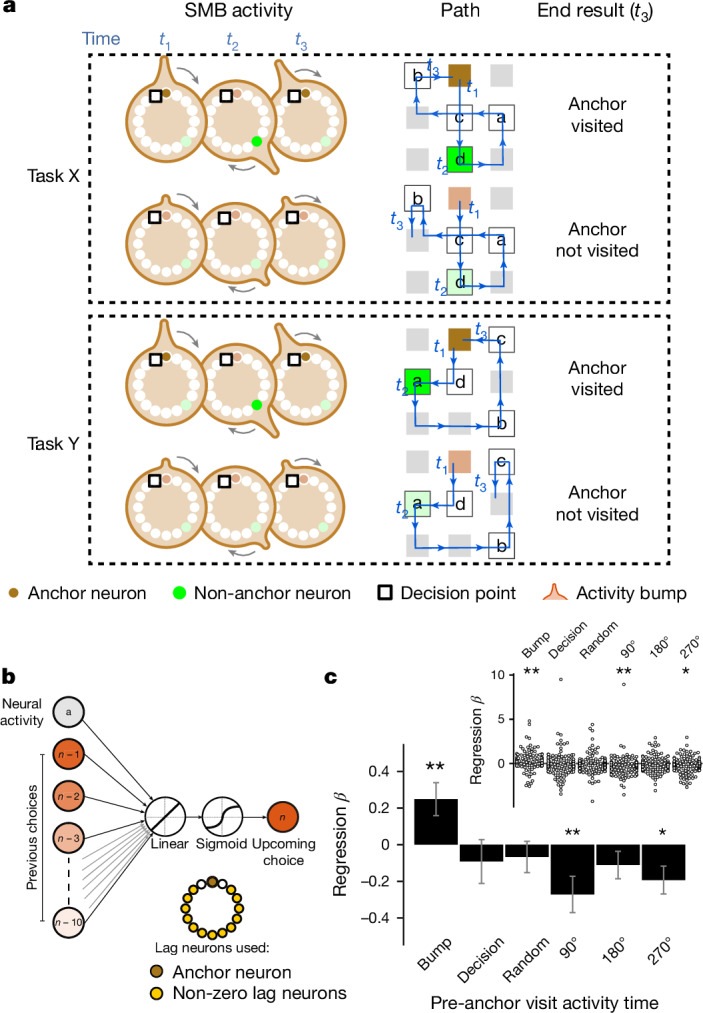
Extended Data Fig. 9. The Structured memory buffers model allows precise and generalisable prediction of future behaviour from neuronal activity.

a) Schematic showing distal prediction of animal’s choices from memory buffers as a function of previous trial choices. By harnessing variability in the coupling between anchor visits and bump initiation, we can test whether SMB activity can predict future choices while controlling for previous choices. In this example we show an SMB with an anchor at location 2 (top middle location shaded in brown) at intermediate goal progress (i.e. half way between goals). Each row shows a different scenario across two consecutive trials (trial N-1 and trial N) in the same task and the expected activity of neurons anchored to this location/goal-progress conjunction. Scenario 1 (0:0): the animal doesn’t visit the anchoring behavioural step in trial N-1 and hence the activity of neurons on this SMB is low. This results in the animal not visiting the anchoring behavioural step in trial N. Scenario 2 (0:1): the animal again doesn’t visit the anchoring behavioural step in trial N-1 but this time the activity of neurons on the SMB is high (e.g. due to noise or top down modulation). This results in the animal visiting the anchoring behavioural step in trial N. Scenario 3 (1:0): the animal visits the anchoring behavioural step in trial N-1 but the activity of neurons on the SMB for this anchor is low (e.g. due to noise or top down modulation). This results in the animal not visiting the anchoring behavioural step in trial N. Scenario 4 (1:1): the animal visits the anchoring behavioural step in trial N-1 and the activity of neurons on the SMB is high. This results in the animal visiting the anchoring behavioural step again in trial N. In effect the variability in the size of the bump in relation to the anchoring behavioural step visit allows us to decouple the SMBs’ activity from previous choices. This makes it possible to test whether SMB activity predicts future choices of the animal. Note that the time stamps shown on the SMB (t1,t2 and t3) are all in trial N. Reproduced/adapted with permission from Gil Costa. b) Prediction of behaviour. Normalised firing rates of neurons during their “bump time”: i.e. the lag at which they are active relative to the anchor. X-axis labels denote visits to a goal-progress/place anchor in the current (N) and upcoming trial (N + 1). For example a value of 0:1 means the anchoring behavioural step was not visited in trial N but visited in trial N + 1. Bump time activity is higher before visits to the neuron’s anchor in trial N + 1 whether the anchoring behavioural step was not visited in trial N (left) or when it was visited in trial N (right). Wilcoxon tests (two-sided): Anchoring behavioural step not visited in trial N: n = 131 tasks, statistic=2749, P = 3.0 × 10⁻⁴. Anchoring behavioural step visited in trial N: n = 123 tasks, statistic=2754, P = 0.008. In addition, an ANOVA on all data (N = 123 tasks) showed a trend towards a main effect of Past F = 3.51 P = 0.063, df1 = 1, df2 = 122, a main effect of Future F = 6.06 P = 0.015, df1 = 1, df2 = 122 and no Past x Future interaction F = 0.80 P = 0.373, df1 = 1, df2 = 122. Scatter plots showing individual points of the same data are shown next to each of the bar plots. c) Regression coefficients were positive for neuronal activity at the “bump time” and also for previous behavioural choices, gradually decreasing with trials in the past. T-tests (two-sided) against 0: “bump time”: N = 131 tasks, statistic=2.74, P = 0.007, df = 130;“n-1”: N = 131, statistic=7.39, P = 1.60 × 10⁻¹³, df = 130; “n-2” N = 131, statistic=8.03 P = 5.04 × 10⁻¹³, df = 130; “n-3” N = 131, statistic = 4.77 P = 4.80 × 10⁻⁶, df = 130; “n-4” N = 131, statistic=3.38, P = 9.45 × 10⁻⁴, df = 130; “n-5” N = 131, statistic=4.36, P = 2.58 × 10⁻⁵, df = 130;“n-6”: N = 131, statistic=1.76, P = 0.080, df = 130; “n-7” N = 131, statistic=2.83 P = 0.005, df = 130; “n-8” N = 131, statistic=2.19 P = 0.030, df = 130; “n-9” N = 131, statistic=2.42, P = 0.017, df = 130; “n-10” N = 131, statistic=0.40, P = 0.691, df = 130. Inset: swarm plots showing distribution of regression coefficient values across groups. d) Prediction of behaviour using neurons anchored at distal points (one state away or more) from the anchor. Top: Normalised firing rates of neurons during their “bump time”: i.e. the lag at which they are active relative to the anchor. Bump time activity is not higher before visits to the neuron’s anchoring behavioural step in trial N + 1 when the anchoring behavioural step was not visited in trial N (Top left) but was higher before visits to anchoring behavioural step in trial N + 1 when the anchoring behavioural step was visited in trial N (Top right). Wilcoxon tests (two-sided): Anchoring behavioural step not visited in trial N: n = 128 tasks, statistic=2917, P = 0.004. Anchoring behavioural step visited in trial N: n = 115 tasks, statistic=2534, P = 0.025. In addition, an ANOVA on all data (N = 115 tasks) showed no main effect of Past: F = 2.43, P = 0.122, df1 = 1, df2 = 114, a main effect of Future: F = 5.74, P = 0.018, df1 = 1, df2 = 114, no Past x Future interaction: F = 0.33, P = 0.566, df1 = 1, df2 = 114. Scatter plots showing individual points of the same data are shown next to each of the bar plots. Bottom left: A logistic regression showed significantly positive coefficients for the bump time but not all other control times. T-tests (two-sided) against 0: “bump time”: N = 128 tasks, statistic=3.68, P = 0.0, df = 127; “decision time”: N = 128 tasks, statistic = −0.56, P = 0.577, df = 127; “random time”: N = 128 tasks, statistic = −0.29, P = 0.769, df = 127; “90 degree shifted time”: N = 128 tasks, statistic = −1.61, P = 0.111, df = 127; “180 degree shifted time”: N = 128 tasks, statistic = −0.61, P = 0.543, df = 127; “270 degree shifted time”: N = 128 tasks, statistic = −2.75, P = 0.007, df = 127. Bottom right: swarm plots showing distribution of regression coefficient values across groups. e) Prediction of behaviour to intermediate (non-rewarded) locations i.e. excluding choices to reward locations. Top: Normalised firing rates of neurons during their “bump time”: i.e. the lag at which they are active relative to the anchor. Bump time activity is higher before visits to the neuron’s anchoring behavioural step in trial N + 1 when the anchoring behavioural step was not visited in trial N (Top left). Wilcoxon tests (two-sided): Anchoring behavioural step not visited in trial N: n = 126 tasks, statistic=2967, P = 0.011. Anchoring behavioural step visited in trial N: n = 120 tasks, statistic=3509, P = 0.751. In addition, an ANOVA on all data (N = 120 tasks) showed no main effect of Past: F = 1.77 P = 0.186, df1 = 1, df2 = 119, no effect of Future: F = 1.37 P = 0.244, df1 = 1, df2 = 119 and no Past x Future interaction F = 0.955 P = 0.330 df1 = 1, df2 = 119. Bottom left: A logistic regression showed coefficients were not significantly positive for any times. T-tests (two-sided) against 0: “bump time”: N = 126 tasks, statistic=1.6, P = 0.112, df = 125; “decision time”: N = 126 tasks, statistic = −2.18, P = 0.031, df = 125; “random time”: N = 126 tasks, statistic = −1.76, P = 0.081, df = 125; “90 degree shifted time”: N = 126 tasks, statistic = −0.54, P = 0.593, df = 125; “180 degree shifted time”: N = 126 tasks, statistic = −0.6, P = 0.552, df = 125; “270 degree shifted time”: N = 126 tasks, statistic = −1.93, P = 0.056, df = 125. Bottom right: swarm plots showing distribution of regression coefficient values across groups. f) Prediction of behaviour to intermediate (non-rewarded) locations i.e. excluding choices to reward locations using Anchor x Task as Ns. Top: Normalised firing rates of neurons during their “bump time”: i.e. the lag at which they are active relative to the anchor. Bump time activity is higher before visits to the neuron’s anchor in trial N + 1 when the anchoring behavioural step was not visited in trial N (Top left) and when it is visited in trial N (Top right). Anchoring behavioural step not visited in trial N: n = 821 anchor-tasks, statistic=154018, P = 0.031. Anchoring behavioural step visited in trial N: n = 529 anchor-tasks, statistic=61812, P = 0.045. In addition, an ANOVA on all data (N = 529 anchor-tasks) showed no main effect of Past: F = 2.66, P = 0.104, df1 = 1, df2 = 526, a trend towards a main effect of Future: F = 2.92, P = 0.088, df1 = 1, df2 = 526, no Past x Future interaction: F = 0.97, P = 0.325, df1 = 1, df2 = 526. Bottom left: A logistic regression showed coefficients were significantly positive for “bump time” but not other times. T-tests (two-sided) against 0: “bump time”: N = 824 anchor-tasks, statistic=2.65, P = 0.008, df = 823; “decision time”: N = 824 anchor-tasks, statistic = −3.12, P = 0.002, df = 823; “random time”: N = 824 anchor-tasks, statistic=0.0, P = 0.998, df = 823; “90 degree shifted time”: N = 824 anchor-tasks, statistic = −3.48, P = 0.001, df = 823; “180 degree shifted time”: N = 824 anchor-tasks, statistic = −0.33, P = 0.744, df = 823; “270 degree shifted time”: N = 824 anchor-tasks, statistic = −2.47, P = 0.014, df = 823. Bottom right: Kernel density estimate plots showing distribution of regression coefficient values across groups. g) Prediction of behaviour to intermediate (non-rewarded) locations i.e. excluding choices to reward locations using all non-zero lag neurons (i.e. not only consistently anchored ones as in all other plots). Top: Normalised firing rates of neurons during their “bump time”: i.e. the lag at which they are active relative to the anchor. Bump time activity is higher before visits to the neuron’s anchoring behavioural step in trial N + 1 when the anchoring behavioural step was visited in trial N (Top right). Wilcoxon tests (two-sided): Anchoring behavioural step not visited in trial N: n = 130 tasks, statistic=3565, P = 0.108. Anchoring behavioural step visited in trial N: n = 130 tasks, statistic=3287, P = 0.024. In addition, an ANOVA on all data (N = 130 tasks) showed no main effect of Past: F = 1.99, P = 0.161, df1 = 1, df2 = 129, no main effect of Future: F = 1.88, P = 0.173, df1 = 1, df2 = 129, no Past x Future interaction: F = 2.11, P = 0.149, df1 = 1, df2 = 129. Bottom left: A logistic regression showed coefficients were significantly positive for “bump time” but not other times. T-tests (two-sided) against 0: “bump time”: N = 130 tasks, statistic=2.08, P = 0.039, df = 129; “decision time”: N = 130 tasks, statistic = −2.83, P = 0.005, df = 129; “random time”: N = 130 tasks, statistic = −0.84, P = 0.402, df = 129; “90 degree shifted time”: N = 130 tasks, statistic = −4.16, P = 5.95 × 10⁻⁵, df = 129; “180 degree shifted time”: N = 130 tasks, statistic = −0.35, P = 0.728, df = 129; “270 degree shifted time”: N = 130 tasks, statistic = −3.18, P = 0.002, df = 129. Bottom right: Swarm plots showing distribution of regression coefficient values across groups. h) Prediction of behaviour to intermediate (non-rewarded) locations i.e. excluding choices to reward locations using all non-zero lag neurons (i.e. not only consistently anchored ones as in all other plots) and using Anchor x Task as Ns. Top: Normalised firing rates of neurons during their “bump time”: i.e. the lag at which they are active relative to the anchor. Bump time activity is higher before visits to the neuron’s anchoring behavioural step in trial N + 1 when the anchoring behavioural step was visited in trial N (Top right) and showed a trend towards being higher when the anchor wasn’t visited in trial N (Top left). Anchoring behavioural step not visited in trial N: n = 1273 anchor-tasks, statistic=380465, P = 0.063. Anchoring behavioural step visited in trial N: n = 826 anchor-tasks, statistic=141977, P = 8.36 × 10⁻⁵. In addition, an ANOVA on all data (N = 826 anchor-tasks) showed a main effect of Past: F = 4.66, P = 0.031, df1 = 1, df2 = 821, a main effect of Future: F = 6.65, P = 0.010, df1 = 1, df2 = 821, a Past x Future interaction: F = 5.38, P = 0.021, df1 = 1, df2 = 821. Bottom left: A logistic regression showed coefficients were significantly positive for “bump time” but not other times. T-tests (two-sided) against 0: “bump time”: N = 1278 anchor-tasks, statistic=3.23, P = 0.001, df = 1277; “decision time”: N = 1278 anchor-tasks, statistic = −3.52, P = 4.39 × 10⁻⁴, df = 1277; “random time”: N = 1278 anchor-tasks, statistic = −1.79, P = 0.073, df = 1277; “90 degree shifted time”: N = 1278 anchor-tasks, statistic = −5.16, P = 2.92 × 10⁻⁷, df = 1277; “180 degree shifted time”: N = 1278 anchor-tasks, statistic = −0.37, P = 0.709, df = 1277; “270 degree shifted time”: N = 1278 anchor-tasks, statistic = −4.37, P = 1.36 × 10⁻⁵, df = 1277. Bottom right: Kernel density estimate plots showing distribution of regression coefficient values across groups. i) Prediction of behaviour in the ABCDE tasks. Top: Normalised firing rates of neurons during their “bump time”: i.e. the lag at which they are active relative to the anchor. Bump time activity is higher before visits to the neuron’s anchor in trial N + 1 when the anchoring behavioural step was not visited in trial N (Top left) and also higher before visits to anchoring behavioural step in trial N + 1 when the anchoring behavioural step was visited in trial N (Top right). Wilcoxon tests (two-sided): Anchoring behavioural step not visited in trial N: n = 24 tasks, statistic=73, P = 0.027. Anchoring behavioural step visited in trial N: n = 24 tasks, statistic=48, P = 0.003. In addition, an ANOVA on all data (N = 24 tasks) showed a main effect of Past: F = 18.57, P = 2.61 × 10⁻⁴, df1 = 1, df2 = 23, a main effect of Future: F = 19.9, P = 1.78 × 10⁻⁴, df1 = 1, df2 = 23, a Past x Future interaction: F = 5.84, P = 0.024, df1 = 1, df2 = 23. Bottom left: A logistic regression showed coefficients were positive for the bump time but not all other control times. T-tests (two-sided) against 0: “bump time”: N = 24 tasks, statistic=2.91, P = 0.008, df = 23; “decision time”: N = 24 tasks, statistic = −1.17, P = 0.252, df = 23; “random time”: N = 24 tasks, statistic = −1.33, P = 0.197, df = 23; “72 degree shifted time”: N = 24 tasks, statistic = −1.97, P = 0.061, df = 23; “144 degree shifted time”: N = 24 tasks, statistic = −0.8, P = 0.43, df = 23; “216 degree shifted time”: N = 24 tasks, statistic = −0.83, P = 0.417, df = 23; “288 degree shifted time”: N = 24 tasks, statistic = −0.88, P = 0.390, df = 23. Bottom right: Swarm plots showing distribution of regression coefficient values across groups. All error bars represent the standard error of the mean.

Extended Data Fig. 10. Internally organised mFC activity is consistent across sleep epochs.

a) Regression coefficient values for pairwise circular (left) or forward (right) distance regressed against sleep cross-correlation for co-anchored neurons - T-test (two-sided) relative to 0: circular distance: N = 430 pairs, t = −2.66 P = 0.008, df = 429; forward distance: N = 430 pairs, t = 1.61 P = 0.108, df = 429. b) No significant differences are seen when comparing regression coefficients for circular distance, forward distance and spatial similarity between co-anchored pairs of neurons between pre- and post-task sleep across the whole-session. Comparison of regression coefficients (from GLM in Fig. 7a) for left: circular distance: Welch’s One-sided T-test: t = 0.14, P = 0.892, df = 919), middle: forward distance: Welch’s One-sided T-test: t = 0.21, P = 0.834, df = 919) and right: spatial similarity: Welch’s One-sided T-test: t = 0.02, P = 0.983, df = 919). N = 521 pairs (pre-task sleep) 399 pairs (post-task sleep). c) Comparison between pre- and post-task sleep across different time epochs since the beginning of sleep sessions for regression coefficients of circular distance (left), forward distance (middle) and spatial similarity (right). Unpaired T-test (Welch’s One-sided T-test) results (with Bonferroni correction of p values): Circular distance: 0-10 min post-sleep: N = 512 (pre-task) N = 429 (post-task): t = −0.69, P = 0.870, df = 939. 10-20 min post-sleep: N = 512 (pre-task) N = 429 (post-task): t = −0.05, P = 0.997, df = 939. 20-30 min post-sleep: N = 512 (pre-task) N = 429 (post-task): t = −0.07, P = 0.997, df = 939. Forward distance: 0-10 min post-sleep: N = 512 (pre-task) N = 429 (post-task): t = −1.33, P = 0.459, df = 939. 10-20 min post-sleep: N = 512 (pre-task) N = 429 (post-task): t = 0.19, P = 0.91, df = 939. 20-30 min post-sleep: N = 512 (pre-task) N = 429 (post-task): t = 0.38, P = 0.91, df = 939. Spatial similarity: 0-10 min post-sleep: N = 512 (pre-task) N = 429 (post-task): t = −1.17, P = 0.567, df = 939. 10-20 min post-sleep: N = 512 (pre-task) N = 429 (post-task): t = −1.11, P = 0.567, df = 939. 20-30 min post-sleep: N = 512 (pre-task) N = 429 (post-task): t = 0.11, P = 0.915, df = 939. All error bars represent the standard error of the mean, analytically derived for each regression. As such there are no individual points to report.

References

1. O’Keefe, J. & Dostrovsky, J. The hippocampus as a spatial map. Preliminary evidence from unit activity in the freely-moving rat. Brain Res.34, 171–175 (1971). - PubMed
1. Hafting, T., Fyhn, M., Molden, S., Moser, M.-B. & Moser, E. I. Microstructure of a spatial map in the entorhinal cortex. Nature436, 801–806 (2005). - PubMed
1. Banino, A. et al. Vector-based navigation using grid-like representations in artificial agents. Nature557, 429–433 (2018). - PubMed
1. Behrens, T. E. J. et al. What is a cognitive map? Organizing knowledge for flexible behavior. Neuron100, 490–509 (2018). - PubMed
1. Whittington, J. C. R. et al. The Tolman–Eichenbaum machine: unifying space and relational memory through generalization in the hippocampal formation. Cell183, 1249–1263.e23 (2020). - PMC - PubMed
LinkOut - more resources