. 2024 Oct 23;24(21):6810.
doi: 10.3390/s24216810.

Multi-Objective Design and Optimization of Hardware-Friendly Grid-Based Sparse MIMO Arrays

Affiliations

Multi-Objective Design and Optimization of Hardware-Friendly Grid-Based Sparse MIMO Arrays

Suleyman Gokhun Tanyer et al. Sensors (Basel). .

Abstract

A comprehensive design framework is proposed for optimizing sparse MIMO (multiple-input, multiple-output) arrays to enhance multi-target detection. The framework emphasizes efficient utilization of antenna resources, including strategies for minimizing inter-element mutual coupling and exploring alternative grid-based sparse array (GBSA) configurations by efficiently separating interacting elements. Alternative strategies are explored to enhance angular beamforming metrics, including beamwidth (BW), peak-to-sidelobe ratio (PSLR), and grating lobe limited field of view. Additionally, a set of performance metrics is introduced to evaluate virtual aperture effectiveness and beamwidth loss factors. The framework explores optimization strategies for the partial sharing of antenna elements, specifically tailored for multi-mode radar applications, utilizing the desirability function to enhance performance across various operational modes. A novel machine learning initialization approach is introduced for rapid convergence. Key observations include the potential for peak-to-sidelobe ratio (PSLR) reduction in dense arrays and insights into GBSA feasibility and performance compared to uniform arrays. The study validates the efficacy of the proposed framework through simulated and measured results. The study emphasizes the importance of effective sparse array processing in multi-target scenarios and highlights the advantages of the proposed design framework. The proposed design framework for grid-spaced sparse arrays stands out for its superior efficiency and applicability in processing hardware compared to both uniform and non-uniform arrays.

Keywords: adaptive desirability function; array design and optimization; grating lobe-free arrays; grid-based sparse MIMO arrays; machine learning; mitigation of mutual coupling; sidelobe reduction.


Conflict of interest statement

The authors declare no conflicts of interest.

Figures

Figure 1
Figure 1
Classification of antenna arrays in terms of inter-element spacing values.
Figure 2
Figure 2
Problem geometry for a planar antenna aperture.
Figure 3
Figure 3
Examples for physical and virtual arrays. (a) The physical elements for 4 TX, 2 RX ULA antenna arrays, (b) 8 element virtual ULA created by the elements given in (a). (c) The physical elements for 8 TX, 9 RX URA antenna arrays, and (d) corresponding fully populated 2D URA virtual array of 72 elements located on the reference grid space. Two other examples for virtual arrays, (e) a non-uniform, and (f) grid-based virtual sparse arrays, respectively (physical locations are ignored).
Figure 4
Figure 4
(a) Uniformly sampled spatial variables, and (b) the corresponding real angles for which (u2 + v2) ≤ 1 is satisfied.
Figure 5
Figure 5
Uniform linear arrays (ULA), dλ = 0.5, (dashed) N = 8, (dashed dot) N = 16, and some examples to (dotted) a sparse array (SA) with dλ = 0.5, and N = 8 with nonuniform positions dλ = 0, 1.07, 2.52, 3.79, 4.48, 4.98, 5.86, 7.5, and (solid) a grid-based sparse array (GSA) with dλ = 0.5, and N = 8 using the positions of as reference for which are thinned to 0, 3, 5, 7, 8, 10, 14, and 15. This figure shows how the main lobe is spread when the array is thinned.
Figure 6
Figure 6
Grating lobe angles with respect to the target angle. (a,b) grating lobes with respect to the target angle for a ULA with dλ = 3λ/2, (c,d), angular separation between the first grating lobe angle, ugl1, and the target angle, ut, for various inter-element spacings where the dotted reference line shows the locus of target angles, ϕ=ϕt0, for which the first phase-wrapped target image appears on the opposite side of the uFOV at ϕ=ϕt0. All values given in the vertical axes carry the angles (left) represented in the (u, v) plane, and (right) given in degrees, respectively. Note that for (c,d) there is no grating lobe for d = λ/2.
Figure 7
Figure 7
Example array structures with mutual coupling forbidden zones, (left) physical apertures for (red) TX and (blue) for RX where the opposite also yields the same VRXs, and (right) their virtual apertures, (a,b) fully-populated URA with no forbidden zones and co-located TX and RXs, (c,d) two-vertical, (e,f) two-diagonal, (g,h) four-corners and (i,j) thick-L shaped, (k,l) wrap-around, and (m,n) improved four corner structures, respectively. Forbidden distances, ymc and zmc are selected to be 15λ and 10λ, respectively.
Figure 7
Figure 7
Example array structures with mutual coupling forbidden zones, (left) physical apertures for (red) TX and (blue) for RX where the opposite also yields the same VRXs, and (right) their virtual apertures, (a,b) fully-populated URA with no forbidden zones and co-located TX and RXs, (c,d) two-vertical, (e,f) two-diagonal, (g,h) four-corners and (i,j) thick-L shaped, (k,l) wrap-around, and (m,n) improved four corner structures, respectively. Forbidden distances, ymc and zmc are selected to be 15λ and 10λ, respectively.
Figure 8
Figure 8
PSLR as a function of sparsity for ULAs with aperture lengths of 16λ, 32λ, 64λ, and 128λ.
Figure 9
Figure 9
Single and two-variable LTB desirability functions, (a) linear, nonlinear (sigmoid function) and piece-wise linear functions with different weights, (b) DPSLR and DBW for γPSLR=2, and γBW=0.5, and (c) D0=DPSLRDBW. Desired regions are assumed to be 40 dB<PSLR<10 dB, and 0.25°<BW<2°.
Figure 9
Figure 9
Single and two-variable LTB desirability functions, (a) linear, nonlinear (sigmoid function) and piece-wise linear functions with different weights, (b) DPSLR and DBW for γPSLR=2, and γBW=0.5, and (c) D0=DPSLRDBW. Desired regions are assumed to be 40 dB<PSLR<10 dB, and 0.25°<BW<2°.
Figure 10
Figure 10
Received signal patterns for uniform linear MIMO arrays with different parameters; (a) Nvrx = 121, d = λ/2, (b) Nvrx = 61, d = λ/2, (c) Nvrx = 61, d = λ.
Figure 10
Figure 10
Received signal patterns for uniform linear MIMO arrays with different parameters; (a) Nvrx = 121, d = λ/2, (b) Nvrx = 61, d = λ/2, (c) Nvrx = 61, d = λ.
Figure 11
Figure 11
Received normalized signal patterns in decibels for a uniform rectangular MIMO array; (Mvrx, Nvrx) = (121, 61), d = λ/2, (a) (ϕt, θt) = (0, 0), (b) (ϕt, θt) = (0, 30°), (c) close up view of the beam width region.
Figure 11
Figure 11
Received normalized signal patterns in decibels for a uniform rectangular MIMO array; (Mvrx, Nvrx) = (121, 61), d = λ/2, (a) (ϕt, θt) = (0, 0), (b) (ϕt, θt) = (0, 30°), (c) close up view of the beam width region.
Figure 12
Figure 12
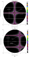
Grid-based sparse arrays, dy = λ/2, dz = λ, wtx = wrx = 2λ, htx = hrx = 5λ, no forbidden zones are defined. (left) Ankara–1A, (right) Ankara–1B, (a,b) Physical element positions where Ankara–1A is utilizing all elements whereas for Ankara–1B the first 8 RXs are disabled, (ch) 2D and 1D received signal patterns in the (u, v) planes with tick values converted to degrees. Single target angles, (ϕt, θt), are (30°, 30°), and (0°, 0°) for 2D and 1D plots, respectively.
Figure 12
Figure 12
Grid-based sparse arrays, dy = λ/2, dz = λ, wtx = wrx = 2λ, htx = hrx = 5λ, no forbidden zones are defined. (left) Ankara–1A, (right) Ankara–1B, (a,b) Physical element positions where Ankara–1A is utilizing all elements whereas for Ankara–1B the first 8 RXs are disabled, (ch) 2D and 1D received signal patterns in the (u, v) planes with tick values converted to degrees. Single target angles, (ϕt, θt), are (30°, 30°), and (0°, 0°) for 2D and 1D plots, respectively.
Figure 13
Figure 13
Inter-element mutual coupling between the transmitter and receiver groups for the sparse array Ankara-1. (a,b) calculated mutual coupling values, (+) K > −60 dB, (o) K < −60 dB.
Figure 14
Figure 14
Mutual coupling constrained grid-based sparse arrays, dy = dz = d = λ/2, wtx = wrx = 2λ, htx = hrx = 5λ, the forbidden distances, ymc = 10λ, and zmc = 15λ. (left) Ankara–2A, (right) Ankara–2B, (a,b) Physical element positions where Ankara–2A is utilizing all elements whereas for Ankara–2B the first 8 RXs are disabled, (ch) optimized 2D and 1D received signal patterns in the (u, v) planes with tick values converted to degrees. Single target angles, (ϕt, θt), are (30°, 30°), and (0°, 0°) for 2D and 1D plots, respectively.
Figure 14
Figure 14
Mutual coupling constrained grid-based sparse arrays, dy = dz = d = λ/2, wtx = wrx = 2λ, htx = hrx = 5λ, the forbidden distances, ymc = 10λ, and zmc = 15λ. (left) Ankara–2A, (right) Ankara–2B, (a,b) Physical element positions where Ankara–2A is utilizing all elements whereas for Ankara–2B the first 8 RXs are disabled, (ch) optimized 2D and 1D received signal patterns in the (u, v) planes with tick values converted to degrees. Single target angles, (ϕt, θt), are (30°, 30°), and (0°, 0°) for 2D and 1D plots, respectively.
Figure 15
Figure 15
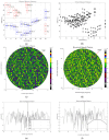
Measured received signal pattern for Ankara–2A with a single target at broadside.
Figure 16
Figure 16
The empirical cumulative distribution functions (ECDF) for the horizontal inter-element spacings of virtual arrays with physical antenna elements of width λ. (a) Horizontal ULA with the number of elements of 16 and 64, and (b) the grid-based sparse Ankara arrays with versions A and B.
Figure 16
Figure 16
The empirical cumulative distribution functions (ECDF) for the horizontal inter-element spacings of virtual arrays with physical antenna elements of width λ. (a) Horizontal ULA with the number of elements of 16 and 64, and (b) the grid-based sparse Ankara arrays with versions A and B.

References

    1. Zheng Z., Wang W., Kong Y., Zhang Y.D. MISC array: A new sparse array design achieving increased degrees of freedom and reduced mutual coupling effect. IEEE Trans. Signal Process. 2019;67:1728–1741. doi: 10.1109/TSP.2019.2897954. - DOI
    1. Krim H., Viberg M. Two decades of array signal processing research: The parametric approach. IEEE Signal Process. Mag. 1996;13:67–94. doi: 10.1109/79.526899. - DOI
    1. Liao B., Madanayake A., Agathoklis P. Array signal processing and systems. Multidim. Syst. Sign. Process. 2018;29:467–473. doi: 10.1007/s11045-018-0555-7. - DOI
    1. Catreux S., Driessen P.F., Greenstein L.J. Data throughputs using multiple-input multiple-output (mimo) techniques in a noise-limited cellular environment. IEEE Trans. Wirel. Commun. 2002;1:226–235. doi: 10.1109/7693.994816. - DOI
    1. Chen Z., Yan F., Qiao X., Zhao Y. Sparse Antenna Array Design for MIMO Radar Using Multiobjective Differential Evolution. Int. J. Antennas Propagat. 2016;2016:1747843. doi: 10.1155/2016/1747843. - DOI

LinkOut - more resources