Analysis of behavioral flow resolves latent phenotypes

Abstract

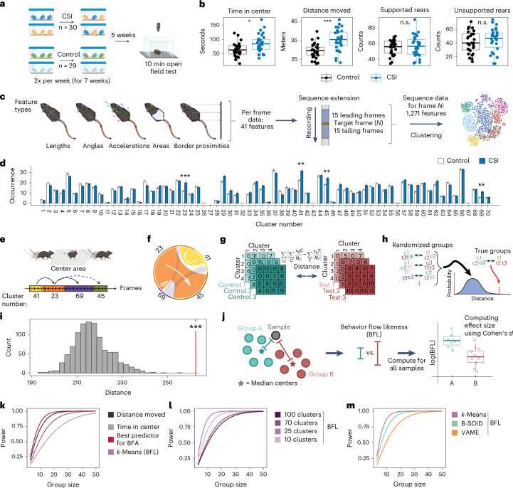
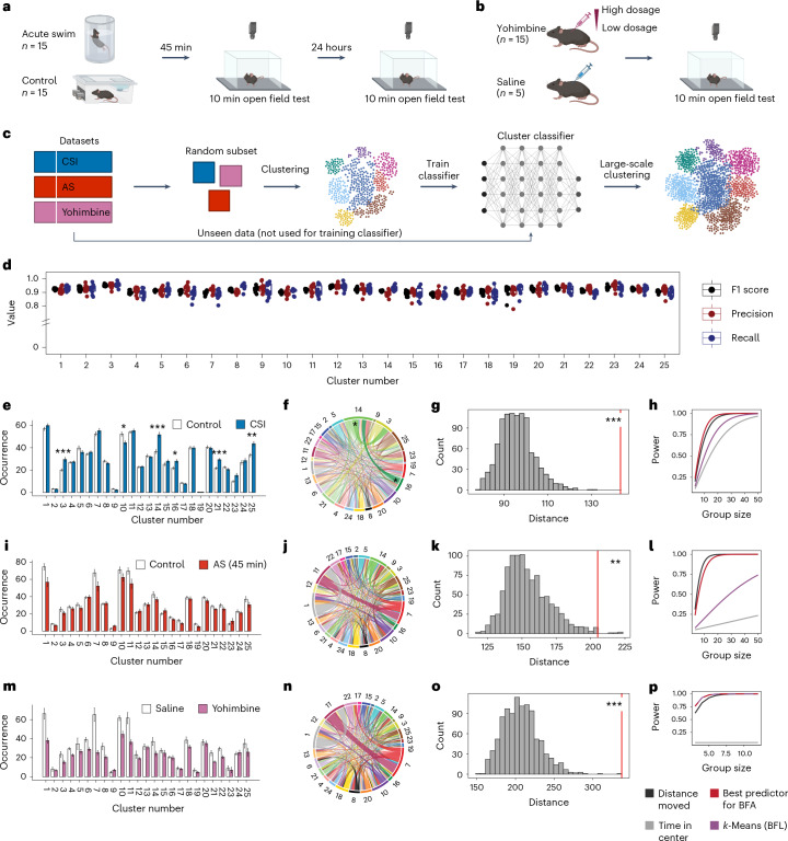
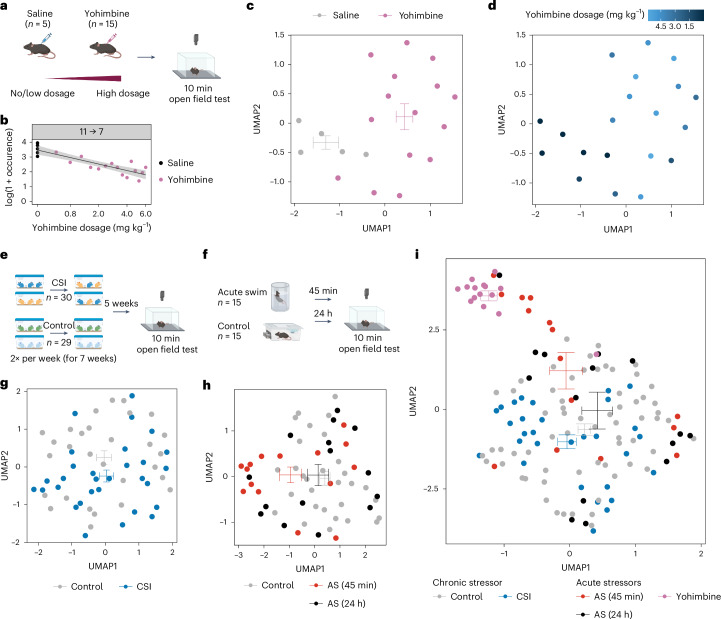
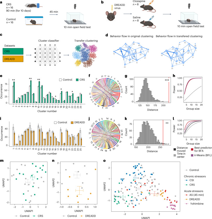
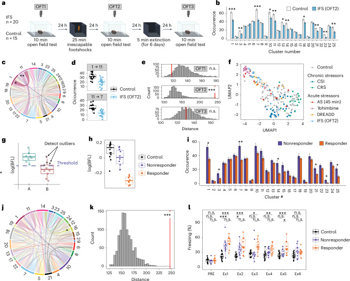
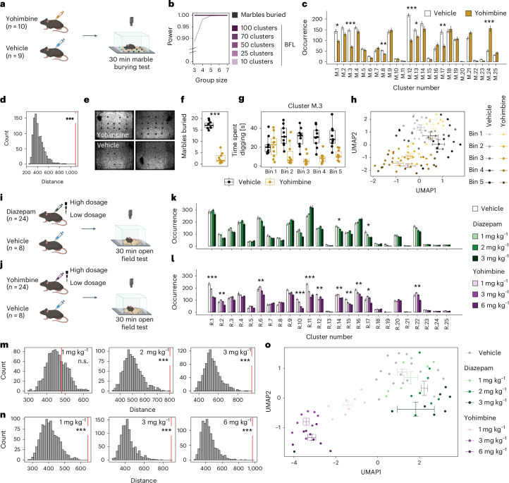
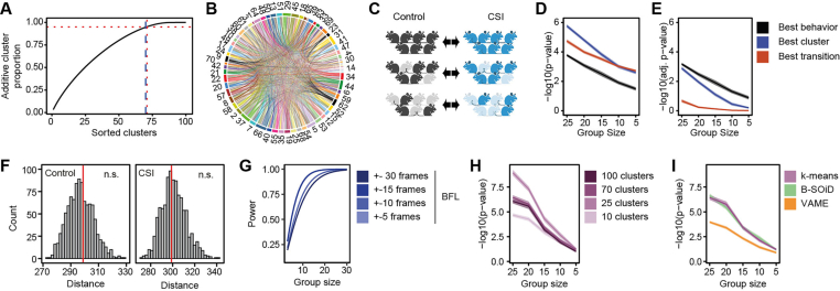
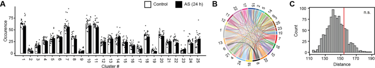
The accurate detection and quantification of rodent behavior forms a cornerstone of basic biomedical research. Current data-driven approaches, which segment free exploratory behavior into clusters, suffer from low statistical power due to multiple testing, exhibit poor transferability across experiments and fail to exploit the rich behavioral profiles of individual animals. Here we introduce a pipeline to capture each animal's behavioral flow, yielding a single metric based on all observed transitions between clusters. By stabilizing these clusters through machine learning, we ensure data transferability, while dimensionality reduction techniques facilitate detailed analysis of individual animals. We provide a large dataset of 771 behavior recordings of freely moving mice-including stress exposures, pharmacological and brain circuit interventions-to identify hidden treatment effects, reveal subtle variations on the level of individual animals and detect brain processes underlying specific interventions. Our pipeline, compatible with popular clustering methods, substantially enhances statistical power and enables predictions of an animal's future behavior.

Fig. 1. BFA increases power to detect phenotypes.

a, A schematic showing the experimental design for CSI. b, Classical behavior readouts in the OFT show that CSI mice (n = 30) spend more time in the center (two-tailed t-test, t(53) = 2.96, adjusted P = 4.47 × 10⁻²) and travel greater distance (two-tailed t-test, t(52) = 4.55, adjusted P = 7.08 × 10⁻⁴) than controls (n = 29). c, Feature extraction based on pose-estimation tracking and sequential feature integration for subsequent clustering. d, The k-means cluster occurrence in CSI (n = 30, controls: n = 29; two-tailed t-tests with multiple testing correction). e, A schematic example of behavioral flow based on cluster transitions. f, The average behavioral flow over all animals between example clusters. The white arrows display the direction of transition. g, Schematic of computing Manhattan distance to compare behavioral transition matrices between groups. h, The permutation approach used for BFA to compare the transition distance based on the true group assignment versus the randomized group assignment. c, control; t, test. i, BFA reveals a treatment effect for CSI (one-tailed z-test, percentile 99.9, z = 5.72, P = 5.28 × 10⁻⁹, d = 0.97). j, Schematic of computing the BFL score to estimate effect sizes. k, Power analysis comparing classical readouts (‘distance moved’ and ‘time in center’) with analysis of cluster transitions. l, The number of clusters influences power to detect treatment effects. m, Power analysis comparing three different clustering algorithms. P values and adjusted P values are denoted as *<0.05, **<0.01 and ***<0.001; n.s., not significant. For box plots, the center line denotes the median value, while the bounding box delineates the 25th to 75th percentiles. The whiskers represent 1.5 times the interquartile range from the lower and upper bounds of the box. The error bars in the bar plot denote mean ± s.e.m.

Fig. 2. Cluster stabilization enables comparisons across experiments.

a,b, A schematic of the experimental design for OFT after acute swim stress (AS) (a) or after yohimbine injections (b). c, Clustering across large datasets. d, Classifier performance on 10-fold cross-validation for each cluster. e, Quantification of cluster occurrences in CSI (n = 30, controls: n = 29; two-tailed t-tests with multiple testing correction). f, Absolute differences in behavioral flow in control versus CSI. For each cluster, the absolute difference in the observed number of transitions between groups is plotted. g, BFA reveals a treatment effect for CSI (one-tailed z-test, percentile 99.9, z = 6.02, P = 8.63 × 10⁻¹⁰, d = 0.92). h, Power analysis in CSI. i, Cluster occurrences in AS (45 min) (n = 15, controls: n = 15; two-tailed t-tests with multiple testing correction). j, The absolute difference in behavioral flow in control versus AS (45 min). k, BFA reveals a treatment effect for AS at 45 min (one-tailed z-test, percentile 99.4, z = 3.09, P = 1.01 × 10⁻³, d = 0.53). l, Power analysis in AS. m, Cluster occurrences in yohimbine (n = 15, controls: n = 5; two-tailed t-tests with multiple testing correction). n, The absolute difference in behavioral flow in saline versus yohimbine. o, BFA reveals a treatment effect for yohimbine (one-tailed z-test, percentile 99.8, z = 5.56, P = 1.38 × 10⁻⁸, d = 2.91). p, Analysis of cluster transitions shows higher power in detecting treatment effects for yohimbine. P values and adjusted P values are denoted as *<0.05, **<0.01 and ***<0.001. The error bars in the bar plots denote mean ± s.e.m.

Fig. 3. BFF captures individual differences in high-dimensional space.

a, A schematic of the experimental design showing the escalating dose of yohimbine. b, Using dose in a log-linear model reveals one significant transition (linear regression, R² = 0.75, F(1,18) = 55.44, adjusted P = 1.64 × 10⁻³). The gray band shows the 95% confidence interval. c, BFF reveals a separation between mice treated with vehicle (n = 5) versus yohimbine (n = 15) when applying UMAP dimension reduction to their transition matrices. d, BFF can also visualize the drug dose delivered to each animal. e, A schematic of the experimental design of the CSI experiment. g, BFF applied to the CSI (n = 30, controls: n = 29) dataset. f, A schematic of the experimental design of the acute swim (AS) stress experiment. h, BFF applied to the acute swim stress (n = 15 at each time point), controls: n = 15) dataset. i, Plotting BFF embeddings across all three experiments (CSI: n = 30, AS: n = 15 (at each time point), yohimbine: n = 15, controls (combined): n = 49) reveals a separation of all experimental groups in 2D space. For every UMAP embedding, the crossbars represent the average UMAP1 and UMAP2 values with s.e.m. for each group.

Fig. 4. Clustering is transferable to new datasets with the same experimental setup.

a,b, A schematic of the experimental design for OFT after CRS (a) or after DREADD activation of the locus coeruleus (b). c, Cluster transfer to new datasets that were not used for the initial clustering. d, Comparison of average behavioral flow in control animals reveals a similar pattern between original clustering (left; CSI, acute swim stress (AS) and yohimbine) and transferred clustering (right; CRS and DREADD). Only transitions with an average appearance >5 are shown. e, Quantification of cluster occurrences in CRS (n = 16, controls: n = 16; two-tailed t-tests with multiple testing correction). f, The absolute differences in behavioral flow in control versus CRS. g, BFA reveals a treatment effect for CRS (one-tailed z-test, percentile 99.9, z = 5.41, P = 3.18 × 10⁻⁸, d = 1.81). h, Power analysis for the CRS experiment. i, Quantification of cluster occurrences after DREADD activation of the locus coeruleus (DREADD: n = 8, controls: n = 8; two-tailed t-tests with multiple testing correction). j, Absolute differences in behavioral flow in saline versus clozapine. k, BFA reveals a treatment effect for the DREADD experiment (one-tailed z-test, percentile 99.2, z = 2.91, P = 1.81 × 10⁻³, d = 1.58). l, Power analysis for the DREADD experiment. m,n, BFF using dimensionality reduction for the CRS experiment (CRS: n = 16, controls: n = 16) (m) and for the DREADD experiment (DREADD: n = 8, controls: n = 8) (n). o, BFF embeddings across original (CSI: n = 30, AS: n = 15, yohimbine: n = 15) and new (CRS: n = 16, DREADD: n = 8, controls (combined): n = 73) experiments. P values and adjusted P values are denoted as *<0.05, **<0.01 and ***<0.001. The error bars in the bar plots denote mean ± s.e.m. For every UMAP embedding, the crossbars represent the average UMAP1 and UMAP2 values with s.e.m. for each group.

Fig. 5. BFF captures individual variability and allows behavioral predictions.

a, A schematic of the experimental design for IFS. b, Cluster occurrences in IFS (OFT2: n = 20, controls: n = 15; two-tailed t-tests with multiple testing correction). c, The absolute difference in behavioral flow in control versus IFS (OFT2). d, Significant transition occurrences in control (n = 15) versus IFS (OFT2, n = 20). e, BFA reveals a treatment effect of IFS only during OFT2 (one-tailed z-test, OFT1: percentile 3.9, z = −1.54, P = 9.39 × 10⁻¹; OFT2: percentile 99.9, z = 7.77, P = 3.89 × 10⁻¹⁵, d = 1.63; OFT3: percentile 44.5, z = −0.18, P = 5.70 × 10⁻¹). f, 2D embedding of behavioral flow across all datasets (CSI: n = 30, AS: n = 15, yohimbine: n = 15, CRS: n = 16, DREADD: n = 8, IFS: n = 20, controls (combined): n = 88). The crossbars represent the average UMAP1 and UMAP2 values with s.e.m. for each group. g, A schematic showing the stratification of nonresponding and responding groups based on BFL score. h, log(BFL) scores for control (n = 15), nonresponder (n = 10) and responder (n = 10) animals. i, Cluster occurrences in nonresponding (n = 10) versus responding (n = 10) mice (two-tailed t-tests with multiple testing correction). j, The absolute differences in behavioral flow in responding versus nonresponding mice. k, BFA reveals a group effect between responding and nonresponding mice (one-tailed z-test, percentile 99.9, z = 6.01, P = 9.23 × 10⁻¹⁰, d = 3.34). l, Freezing response before (PRE) IFS exposure and during subsequent extinction sessions (Ex1–6) for control (n = 15), nonresponder (n = 10) and responder (n = 10) mice (two-way ANOVA for general effect, followed by two-tailed t-tests between groups with multiple testing correction). P values and adjusted P values are denoted as *<0.05, **<0.01 and ***<0.001; n.s., not significant. The error bars in the bar plots denote mean ± s.e.m. For box plots, the center line denotes the median value, while the bounding box delineates the 25th to 75th percentiles. The whiskers represent 1.5 times the interquartile range from the lower and upper bounds of the box.

Fig. 6. BFA and BFF are transferable to other setups.

a, A schematic showing the experimental design for the marble burying test (MBT) after yohimbine or vehicle injection. b, Power analysis comparing different numbers of k-means clusters with the number of ‘marbles buried’ for MBT. c, Cluster occurrences in MBT (yohimbine: n = 10, vehicle: n = 9; two-tailed t-tests with multiple testing correction). d, BFA reveals a treatment effect of yohimbine (one-tailed z-test, percentile 99.9, z = 7.1, P = 6.21 × 10⁻¹³, d = 6.57) in MBT. e, Examples of final frames showing marbles buried after yohimbine (top) versus vehicle injection (bottom). f, Marbles buried differ significantly (two-tailed t-test, t(16) = 16.2, P = 2.03 × 10⁻¹¹) after vehicle (n = 9) versus yohimbine (n = 10) injection. g, Time spent in cluster M.3 (digging cluster) evolves differently over time for mice after vehicle (n = 9) or yohimbine (n = 10) injection. Each bin represents 6 min. h, BFF shows change in behavior profile over time for yohimbine (n = 10) and vehicle (n = 9). i, A schematic showing the experimental design for OFT after diazepam or vehicle administration. j, A schematic showing the experimental design for OFT after yohimbine or vehicle injection in another laboratory using a different OFT setup. k,l, Cluster occurrence in diazepam (n = 24, vehicle: n = 8) (k) or in yohimbine (n = 24, vehicle: n = 8; one-way ANOVA with multiple testing correction) (l). m, BFA shows treatment effects after higher doses of diazepam (one-tailed z-test, 1 mg kg⁻¹: percentile 68.93, z = 0.5, P = 3.08 × 10⁻¹; 2 mg kg⁻¹: percentile 99.9, z = 4.14, P = 1.76 × 10⁻⁵, d = 2.72; 3 mg kg⁻¹: percentile 99.9, z = 4.91, P = 4.64 × 10⁻⁷, d = 4.2). n, BFA reveals behavioral changes after different doses of yohimbine injections (one-tailed z-test, 1 mg kg⁻¹: percentile 99.9, z = 4.44, P = 4.52 × 10⁻⁶, d = 4.32; 3 mg kg⁻¹: percentile 99.9, z = 6.1, P = 5.27 × 10⁻¹⁰, d = 6.12; 6 mg kg⁻¹: percentile 99.9, z = 6.37, P = 9.60 × 10⁻¹¹, d = 6.33). o, BFF separates the different doses of diazepam (n = 24) and yohimbine (n = 24) administrations from vehicle injections (combined: n = 16). P values and adjusted P values are denoted as *<0.05, **<0.01 and ***<0.001. The error bars in the bar plots denote mean ± s.e.m. For box plots, the center line denotes the median value, while the bounding box delineates the 25th to 75th percentiles. The whiskers represent 1.5 times the interquartile range from the lower and upper bounds of the box.

Extended Data Fig. 1. BFA increases power to detect phenotypes.

(a) Determining the optimal number of clusters for k-means. Vertical, red-dashed line marks the number of clusters (=71) which represent 95% of all frames (horizontal red-dashed line), and the blue dashed line marks the number of clusters (=70) we used for the CSI analysis. (b) Average behavioral flow for all 70 clusters over all animals. (c) Schematic of in silico approach to generate random subsets of each group of mice to run multiple two-group comparisons while gradually reducing group sizes. (d) Phenotype detection sensitivity in CSI with unadjusted p-values (two-tailed t-test). Cluster usage and cluster transitions were compared against the best statistical value between distance, time in center, supported rearing and unsupported rearing, termed "best behavior". (e) Sensitivity in CSI with adjusted p-values (two-tailed t-test) after appropriate multiple testing correction. (f) BFA shows no differences for only control (one-tailed z-test, percentile=60.3, z=0.2, p=4.19*10⁻¹) or only CSI animals (one-tailed z-test, percentile=45.0, z=−0.2, p=5.78*10⁻¹). (g) Power analysis comparing different integration periods. (h) BFA (one-tailed z-test) enhances sensitivity using various numbers of k-means clusters. (i) Phenotype detection sensitivity in CSI using B-SOiD or VAME clustering with BFA (one-tailed z-test). The bands in each sensitivity plot display ± SEM.

Extended Data Fig. 2. Clustering results in AS after 24 hours.

(a) Cluster occurrences in AS (24 h: n=15, controls: n=15; two-tailed t-tests with multiple testing correction). (b) Absolute difference of behavioral flow in control vs. AS (24 h). (c) BFA does not show treatment effects at 24 h (one-tailed z-test, percentile=80.9, z=0.85, p=0.198). Error bars in the bar plot denote mean ± SEM.

Extended Data Fig. 3. Clustering results in IFS (for OFT1 and OFT3).

(a) Cluster occurrences in IFS (OFT1: n=20, controls: n=15; two-tailed t-tests with multiple testing correction). (b) Absolute difference in behavioral flow in control vs. IFS (OFT1). (c) Cluster occurrences in IFS (OFT3: n=20, controls: n=15; two-tailed t-tests with multiple testing correction). (d) Absolute difference in behavioral flow in control vs. IFS (OFT3). Error bars in the bar plots denote mean ± SEM.

Extended Data Fig. 4. BFA and BFF applied to other behavioral tests and setups.

(a) Schematic showing experimental design for the light-dark box (LDB) test after chronic restraint stress (CRS). (b) Power analysis comparing different numbers of k-means clusters with classical readouts ("transitions" and "time in light") for the LDB test. (c) Cluster occurrences in LDB after CRS (n=16, controls: n=16; two-tailed t-tests with multiple testing correction). (d) BFA reveals a treatment effect of CRS (one-tailed z-test, percentile=99.5, z=3.06, p=1.09*10⁻³, d=0.91) in LDB. (e) BFF applied to LDB data after CRS (n=16, controls: n=16). (f) Schematic showing experimental design for exposure to fear conditioning box. (g) Power analysis comparing different numbers of k-means clusters for fear conditioning box. (h) Cluster occurrences in fear conditioning box (IFS: n=20, controls: n=15; two-tailed t-tests with multiple testing correction). (i) BFA shows a treatment effect of the fear conditioning box (one-tailed z-test, percentile=99.9, z=10.6, p=0, d=5.44). (j) BFF applied to fear conditioning box data (IFS: n=20, controls: n=15). Each bin represents 5 minutes. (k) Comparison of classical behavior readouts for different doses of diazepam (n=24, vehicle: n=8) or yohimbine (n=24, vehicle: n=8) (one-way ANOVA, time in center for diazepam: F(3,28)=0.78, adj. p=5.14*10⁻¹; for yohimbine: F(3,28)=3.2, adj. p=3.84*10⁻²; distance moved for diazepam: F(3,28)=4.09, adj. p=2.62*10⁻²; for yohimbine; F(3,28)=46.27, adj. p=2.81*10⁻¹⁰; supported rears for diazepam: F(3,28)=4.68, adj. p=2.26*10⁻², for yohimbine: F(3,28)=29.18, adj. p=1.53*10⁻⁸; unsupported rears for diazepam: F(3,28)=8.85, adj. p=1.38*10⁻³; for yohimbine: F(3,28)=4.02, adj. p=2.11*10⁻²). (l) Power analysis comparing different numbers of k-means clusters with classical OFT readouts after treatment with diazepam or (m) yohimbine. (n) BFA reveals differences between higher doses of diazepam (2 or 3 mg/kg) compared to lower doses (1 mg/kg) (one-tailed z-test, 1 vs. 2 mg/kg: percentile=96.4, z=2.04, p=2.06*10⁻², d=0.19; 1 vs. 3 mg/kg: percentile=99.7, z=3.34, p=4.15*10⁻⁴, d=1.15; 2 vs. 3 mg/kg: percentile=49.45, z=−0.1, p=5.41*10⁻¹). (o) BFA shows treatment differences between different doses of yohimbine (one-tailed z-test, 1 vs. 3 mg/kg: percentile=99.7, z=3.71, p=1.05*10⁻⁴, d=2.45; 1 vs. 6 mg/kg: percentile=99.8, z=5.68, p=6.82*10⁻⁹, d=5.36; 3 vs. 6 mg/kg: percentile=99.2, z=3.43, p=3.00*10⁻⁴, d=1.49). p-values and adj. p-values are denoted as: *<0.05, **<0.01, ***<0.001. Error bars in the bar plots denote mean ± SEM. For every UMAP embedding, the crossbars represent the average UMAP1 and UMAP2 values with SEM for each group. For box plots, the center line denotes the median value, while the bounding box delineates the 25th to 75th percentiles. Whiskers represent 1.5 times the interquartile range from the lower and upper bounds of the box.

References

1. Kafkafi, N., Yekutieli, D., Yarowsky, P. & Elmer, G. I. Data mining in a behavioral test detects early symptoms in a model of amyotrophic lateral sclerosis. Behav. Neurosci.122, 777–787 (2008). - PubMed
1. Kafkafi, N., Yekutieli, D. & Elmer, G. I. A data mining approach to in vivo classification of psychopharmacological drugs. Neuropsychopharmacology34, 607–623 (2009). - PubMed
1. Lauer, J. et al. Multi-animal pose estimation, identification and tracking with DeepLabCut. Nat. Methods19, 496–504 (2022). - PMC - PubMed
1. Pereira, T. D. et al. SLEAP: a deep learning system for multi-animal pose tracking. Nat. Methods19, 486–495 (2022). - PMC - PubMed
1. Mathis, A. et al. DeepLabCut: markerless pose estimation of user-defined body parts with deep learning. Nat. Neurosci.21, 1281–1289 (2018). - PubMed
LinkOut - more resources