Breast ultrasound knobology and the knobology of twinkling for marker detection

Abstract

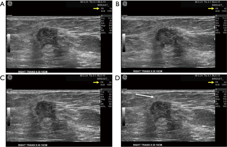
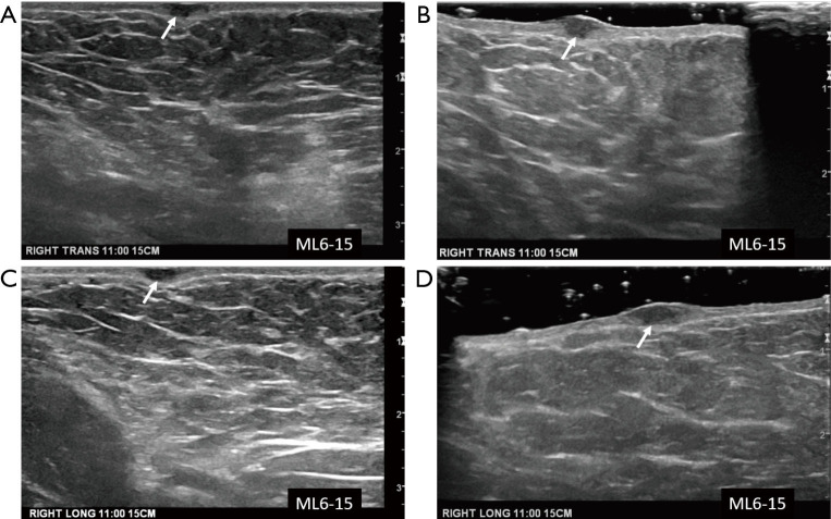
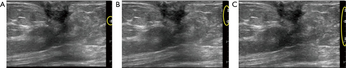
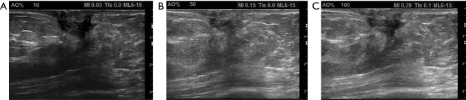
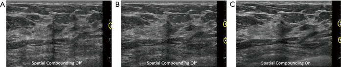
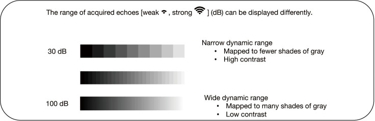
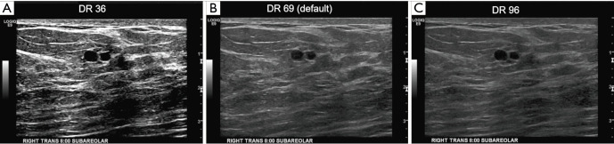
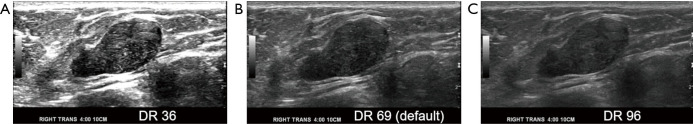
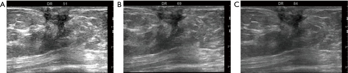
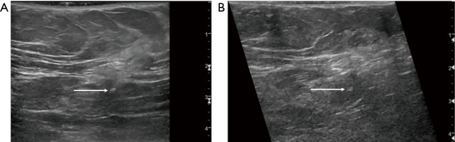
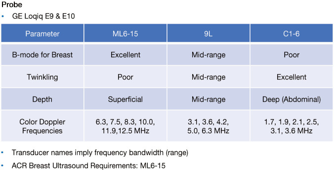
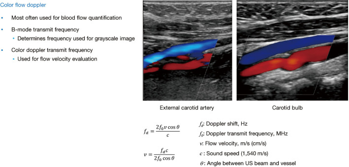
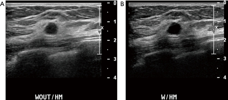
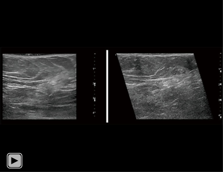
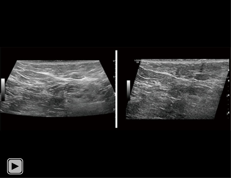
Breast ultrasound utilizes various scanning techniques to acquire optimal images for diagnostic evaluation. During interventional procedures, such as ultrasound-guided biopsies or preoperative localizations, knowledgeable and purposeful scanning adjustments are critical for successfully identifying the targeted mass or biopsy marker or clip. While most ultrasound scanning parameters are similar across different vendors, detailed descriptions specifically addressing the scanning parameters-often referred to as "knobology"- for breast ultrasound is at best limited in the literature. This review highlights ten key operator-controlled adjustments (including transducer selection, beam focusing, power, depth, gain and time gain compensation, harmonic imaging, spatial compounding, dynamic range, beam steering, and color Doppler) that significantly influence image quality in breast ultrasound. Each adjustment is accompanied by an "In practice" section providing examples and practical tips on implementation. The last topic discusses color Doppler which is generally used in breast ultrasound for evaluating the vascularity of a finding. Color Doppler, or more specifically, color Doppler twinkling, can be leveraged as a technique to detect certain breast biopsy markers that are challenging to detect by conventional B-mode ultrasound. While the cause of color Doppler twinkling is still under active investigation, twinkling is a clinically well-known, compelling ultrasound feature typically described with kidney stones. A step-by-step guide on how to use color Doppler twinkling to detect these markers is provided.

Keywords: Breast ultrasound; color Doppler twinkling; knobology; twinkling; ultrasound scanning.

Figure 1

Axial and lateral resolutions. The axial resolution, which is determined by the transmit frequency associated with the array of the piezoelectric crystals, is generally better than the lateral resolution, which is determined by the footprint, application, and transmit frequency. The ultrasound beam (red) emitted along its path (green arrows) from the transducer gets narrowed at the focal zone and then widens with more depth as it sweeps from one end of the transducer to the other (large gray arrow). The axial resolution (blue), equal to half the spatial pulse length, defines to what extent one can separate two close objects or points along the direction of the beam. The lateral resolution varies slightly along the beam’s path. The elevation resolution defines the slice thickness of the imaging plane.

Figure 2

Selection of transducer. A conventional high-frequency transducer for breast ultrasound (ML6-15, GE Logiq E9, GE Healthcare, Wauwatosa, WI, USA) shows a skin finding (A, arrow). Using a higher frequency transducer, such as the L8-18i (B), the details of the skin finding (B, arrow), such as the margins, can be improved. Some of these features are vendor-specific. In this case, the higher frequency transducer provides higher axial and lateral resolution, but there is an overall smoothed pixelated appearance, making it somewhat blurrier than the lower frequency transducer. This could be a vendor-specific observation and can be mitigated by using harmonic imaging.

Figure 3

Focal zones. To improve the lateral resolution of the image, the ultrasound beam (A, gray) can be focused (B, arrow) to improve the lateral resolution at that location (*). Multiple beam-focusing placements (C, arrows) cause an effective column of improved lateral resolution (D), which may improve feature sharpness. (Used with permission by Mayo Foundation for Medical Education and Research, all rights reserved. Original image modified by Christine Lee).

Figure 4

Placement of single focal zones and multiple focal zones. Changing the placement of a single focal zone [A-D hourglass (⧖) symbol on the right-hand side of each image] while keeping all other imaging parameters the same shows subtly improved sharpness near the level of each focal zone. For example, when the focal zone is placed at 1.50 cm deep (A), the tissues at this depth are sharper than when the focal zone is at 3.25 cm (D). In (A-D), each image with a single focal zone had a frame rate of 64 fps, but in (E) with multiple focal zones, the frame rate dropped to 16 fps.

Figure 5

Multiple focal zones. Using an ML6-15 transducer and keeping all other parameters the same, images of this irregular hypoechoic mass were acquired with one to four focal zones [A-D, hourglass (⧖) symbols on the right-hand side of each image]. Imaging differences are subtle with (B) slightly off plane compared to (A,C,D). Utilizing multiple focal zones can help better evaluate tissue characteristics, e.g., a subtle, small, taller-than-wide, isoechoic-hypoechoic mass with irregular and indistinct margins (D, white arrow) when a focal zone near the near field is placed. Note that increasing the focal zones decreases the frame rate (A-D, yellow arrows).

Figure 6

Optimizing focal zones for very superficial findings. This is the same finding shown in Figure 2. Using a high-frequency transducer for conventional breast ultrasound, an ML6-15 in this case, a dermal finding (A,C, arrow) is not at the optimal location relative to the focal zones indicated by the hourglass (⧖) symbols on the right-hand side of the image despite setting the focal zones being at their most superficial locations. Using a thicker layer of gel, the dermal finding can be better placed at the focal zones (B,D, arrow).

Figure 7

When adjusting focal zones shows no appreciable diagnostic change. In this example, the number of focal zones (A-C, yellow) is increased from 1 (A), to 2 (B), to 3 (C). The (⧖) symbols on the right-hand side of each image (yellow circles) indicate the focal zones. When there is no diagnostic value to increasing the focal zones, one could choose to scan with the fewest focal zones as increasing focal zones decreases the frame rate.

Figure 8

Power (acoustic output) knob. In this example, which is the same finding shown in Figure 7, the AO is changed to 10% (A), 50% (B), and 100% (C) while keeping all other scanning parameters constant. Increasing the AO increases the MI and the TI. The default AO is set to 100% (C). AO, acoustic output; MI, mechanical index; TI, thermal index.

Figure 9

Using depth to frame a finding relative to surrounding anatomy. On the CC view, a mammographic finding (A, circle) is within dense fibroglandular tissue (A, arrow) in the middle-depth breast. Ultrasound of the breast shows a dense band of fibroglandular tissue (B, arrow) that is located middle depth between the skin and the pleura. This finding was biopsied using ultrasound-guidance and post-clip mammogram shows the biopsy marker (C, arrow) corresponding to the expected mammographic location (A) and confirming that what was seen on ultrasound corresponds to the mammographic finding. CC, craniocaudal.

Figure 10

Adjusting the gain. With all the other scanning parameters held constant, adjusting the overall gain (A,B, arrows) was performed to assess the relative echogenicity.

Figure 11

Gross anatomy of breast parenchyma. A longitudinal cross-section of cadaveric breast tissue shows the heterogeneity of the tissues from smooth fatty lobules (arrow) to a region of heterogeneous fibroglandular tissues that include suspensory ligaments (of Cooper), ducts, glandular structures, and vasculature (dotted region). Harmonic imaging can be considered when imaging areas of heterogeneous interfaces.

Figure 12

Harmonic imaging for improved sharpness and contrast of parenchymal interfaces. Default conventional breast imaging uses spatial compounding, as seen with the breast cancer in (A, arrow). In (B) harmonic imaging is turned on. Harmonic imaging is referred to as contrast harmonic imaging on the GE Logiq E9 scanner and indicated by the double hourglass icons (⧖⧖) on the right-hand side of the image (B). With harmonic imaging, note the improved sharpness of the interfaces of fatty lobules and the interdigitating fibroglandular tissues (B, circled region). The margins of the mass adjacent to the background breast parenchyma particularly below the white dashed lines in (B) are also sharper.

Figure 13

Harmonic imaging for improved sharpness and contrast of axillary lymph nodes. Improved visualization of a deeper axillary lymph node using the ML6-15 transducer is obtained with harmonic imaging in the longitudinal view (A, white arrow) and in the transverse view (B, white arrow). During fine needle aspiration of this lymph node, harmonic imaging can help confirm correct placement of the needle tip. In (C) harmonic imaging can be used with the L8-18i transducer to identify a different axillary lymph node (C, arrow).

Figure 14

Changing more than one knob. Given this superficial finding (same as the finding in Figures 7,8) with questionable middle-depth involvement (1–2 cm deep) using the ML6-15 transducer (A), a couple of other techniques were attempted. Harmonic imaging (B) increased the radiologist’s confidence in extension of the process to the middle depth, and changing to a higher-frequency transducer (C), the L8-18i, along with harmonic imaging showed persistence of the middle-depth hypoechoic areas which warranted description in the final report.

Figure 15

L8-18i transducer at different transmit frequencies with and without harmonic imaging. Realize that one can also change the transmit frequency for a given transducer. Keeping all other scanning parameters the same, harmonic imaging at a transmit frequency of 15 MHz shows slightly better contrast and margin definition (B,D) than the images acquired without harmonic imaging (A,C). In this case, the L8-18i allowed for a transmit frequency of 18 MHz (E) which combined with harmonic imaging shows good conspicuity of the mass.

Figure 16

Spatial compounding. By default, spatial compounding is turned on. A breast cancer is shown with (A) and without (B) spatial compounding. When spatial compounding is off, the breast parenchyma surrounding the breast cancer, particularly posteriorly, is slightly noisier, a reflection of single image acquisition. Note that the shadowing features without spatial compounding (B) show slightly more contrast to the adjacent tissues when compared to an image acquisition with spatial compounding (A).

Figure 17

Focal zones and spatial compounding. The irregular hypoechoic mass in the center of each image illustrates slight variations with one focal zone (A) versus two focal zones (B,C). A smoother or softer look is appreciated when spatial compounding in turned on (C) as it involves some speckle reduction and frame averaging which is vendor-specific.

Figure 18

Dynamic range. In this illustration, a narrow dynamic range, such as 30 dB, maps the acquired echoes to fewer shades of gray, increasing the contrast of the image. Similarly, a wider dynamic range, such as 100 dB, maps the acquired echoes to more shades of gray, essentially reducing the contrast of the image. This can be appreciated in the horizontal gray bars, where the contrast between the shades of gray is more readily apparent with a narrow dynamic range (30 dB) compared to a wider dynamic range (100 dB).

Figure 19

DR and background echotexture. Holding all other scanning parameters constant, the dynamic range has been varied from the narrowest DR of 36 dB in (A), to the default DR of 69 dB (B), and then to the widest DR of 96 dB (C). The higher contrast is evident with the narrowest DR in (A). Note that in high contrast images (A), the details can be lost in very high signal areas and in very low signal areas. In comparison, very low contrast images (C) can effectively efface heterogeneous echotexture of the background breast parenchyma. DR, dynamic range.

Figure 20

DR and margins. Holding all other scanning parameters constant, the DR has been varied from the narrowest DR of 36 dB in (A), to the default DR of 69 dB (B), and then to the widest DR of 96 dB (C). The high-contrast image with a DR of 36 dB (A) provides some detail of the margins of the mass not well appreciated when the DR is increased (C). Again, with low DR, details are lost in very high signaling areas (A, white areas) and in very low signaling areas (A, black areas). DR, dynamic range.

Figure 21

DR and visualization preferences. The irregular hypoechoic mass shown is the same one in Figures 7,8,14. Holding all other scanning parameters constant, the DR has been varied from a DR of 51 dB in (A), to the default DR of 69 dB (B), and then to a DR of 84 dB (C). Depending on what feature one is focusing on, one can vary the DR knob to provide more contrast to certain areas by lowering the DR. DR, dynamic range.

Figure 22

Steering. These two static images show fine-needle aspiration of an axillary lymph node without (A) and with (B) steering. Steering is evident by the angled field of view (B). For this particular ultrasound vendor, steering requires disabling spatial compounding, so the steered image (B) appears less smooth. Without steering, the default spatial compounding results in a smoother image appearance (B). While the needle tip (A,B, arrow) can be seen without (A) and with (B) beam steering, preference for steering is user dependent. The performance of steering is sometimes better appreciated in cine clips. Two cine clips without and with steering (Videos S1,S2) are provided in the supplemental section.

Figure 23

Twinkling and transducer selection. While color Doppler twinkling is more readily detected using a lower frequency transducer, the anatomic detail in the breast using this transducer will be poor. Immediate subsequent interrogation of the site of twinkling using a higher frequency transducer typically used in breast ultrasound is then performed to identify features of the breast biopsy marker which can be subtle (8). ACR, American College of Radiology.

Figure 24

Twinkling and color flow Doppler. Color Doppler transmit frequency is different than B-mode transmit frequency but is dependent on the B-mode transmit frequency, which is inherent with the transducer selected. For twinkling detection, the operator will need to select a more favorable f₀, which is later described. US, ultrasound.

Figure 25

Twinkling and color Doppler transmit frequency. Twinkling detection is more favorable for lower frequency transducers such as the 9L and the C1–6 transducers, and for each of these transducers, the lower color Doppler transmit frequencies are favored. For the 9L transducer, using a color Doppler transmit frequency ranging 3.1–4.2 MHz is favored; and for the C1–6 transducer, using a color Doppler transmit frequency ranging 1.7–3.1 MHz is favored. One of the characteristics of true twinkling is its insensitivity to changes in color Doppler transmit frequencies (7).

Figure 26

Twinkling and Doppler gain. Doppler GN is operator-dependent and strives to strike a balance between twinkling and noise. The maximum gain on this ultrasound scanner is 30.0. When the GN is set too low (GN =10.0), noise is filtered out but so is a substantial component of twinkling. When the GN is set too high (GN =27.0), noise can confound the twinkling signature. The GN is often selected to just below the level of noise, in this case GN =18.0, that demonstrates twinkling with very minimal, if any, noise. GN, gain; CF, color flow.

Figure 27

Twinkling and color Doppler scale. Twinkling in (A-C) is robust despite changes to the scale ±5 cm/s (A), ±12 cm/s (B), and ±30 cm/s (C).

Figure 28

Color Doppler ultrasound twinkling-detection of markers. Using a curvilinear lower frequency transducer, the C1–6, color Doppler twinkling readily characterizes this biopsy marker, in this case a Tumark Q marker (arrow). Earlier extensive B-mode scanning with the conventional ML6-15 transducer could not identify the marker. Note that the twinkling comet tail (chevron) is also seen.

Figure 29

Comparing knobs to maximize characterization of features. The indistinct margins without harmonic imaging (A) persist with harmonic imaging (B). The hypoechoic internal echogenicity of the mass without harmonic imaging (A) outweighs the harmonic images with through-transmission and apparent anechoic internal characteristics that might suggest a cyst or cystic component. This mass was biopsied and was an invasive ductal carcinoma.

Video S1

This ultrasound cine clip demonstrates a fine-needle aspiration of an axillary lymph node without (left) and with (right) steering. The needle and its tip are seen (arrows).

Video S2

This is another ultrasound cine clip demonstrating a fine-needle aspiration of an axillary lymph node without (left) and with (right) steering. The needle and its tip are seen (arrows).

References

1. Nicosia L, Gnocchi G, Gorini I, et al. History of Mammography: Analysis of Breast Imaging Diagnostic Achievements over the Last Century. Healthcare (Basel) 2023;11:1596. 10.3390/healthcare11111596 - DOI - PMC - PubMed
1. WILD JJ , NEAL D. Use of high-frequency ultrasonic waves for detecting changes of texture in living tissues. Lancet 1951;1:655-7. - PubMed
1. Fornage BD, Toubas O, Morel M. Clinical, mammographic, and sonographic determination of preoperative breast cancer size. Cancer 1987;60:765-71. 10.1002/1097-0142(19870815)60:4<765::AID-CNCR2820600410>3.0.CO;2-5 - DOI - PubMed
1. Lee J. Practical and illustrated summary of updated BI-RADS for ultrasonography. Ultrasonography 2017;36:71-81. 10.14366/usg.16034 - DOI - PMC - PubMed
1. Lee CS, Bohm-Velez M. ACR Practice Parameter for the Performance of a Diagnostic Breast Ultrasound Examination. Am Coll Radiol 2021. Available online: https://www.acr.org/-/media/ACR/Files/Practice-Parameters/US-Breast.pdf