Machine learning enabled fast optical identification and characterization of 2D materials

Abstract

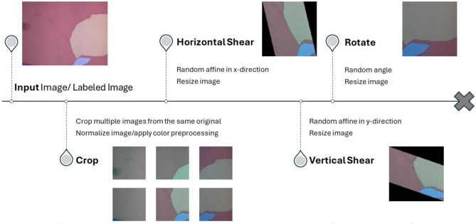
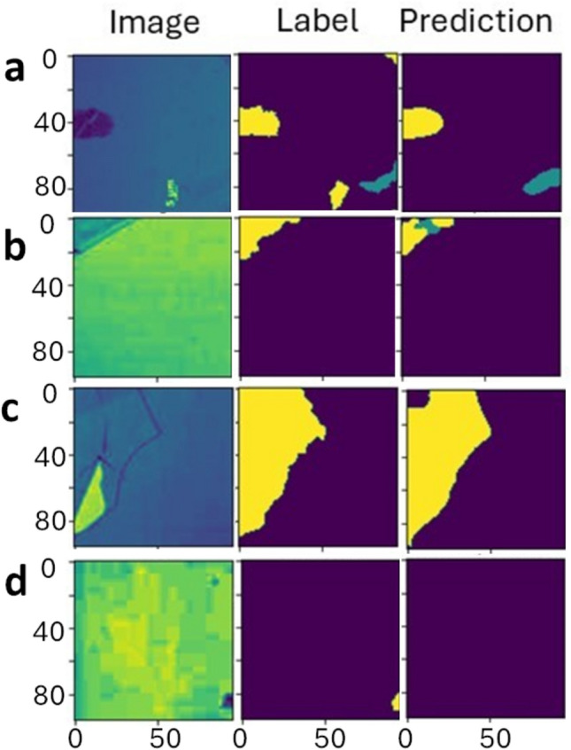
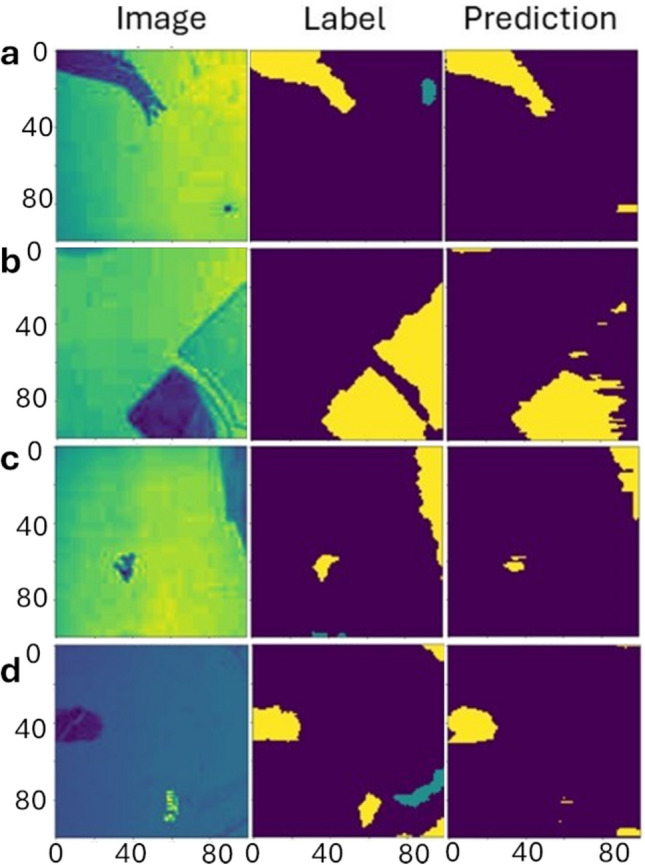
Two-dimensional materials are a class of atomically thin materials with assorted electronic and quantum properties. Accurate identification of layer thickness, especially for a single monolayer, is crucial for their characterization. This characterization process, however, is often time-consuming, requiring highly skilled researchers and expensive equipment like atomic force microscopy. This project aims to streamline the identification process by using machine learning to analyze optical images and quickly determine layer thickness. In this paper, we evaluate the performance of three machine learning models - SegNet, 1D U-Net, and 2D U-Net- in accurately identifying monolayers in microscopic images. Additionally, we explore labeling and image processing techniques to determine the most effective and accessible method for identifying layer thickness in this class of materials.

Fig. 1

Image Preprocessing Techniques. (a) The original image before any preprocessing. The blue line indicates where the contrast measurements were taken from. The scale is missing from the image source but should be $\approx 100\mu m$ in width. (b) The contrast measurements along the blue line in the original image. The edges of the material are clearly demarcated by large jumps in contrast. (c) L*a*b* diagram with lightness information indicated by color and color information indicated by position: +a* for the red direction, -a* for the green direction, +b* for the yellow direction, and -b* for the blue direction. (d) RGB diagram with R and G for red and green color intensity and B for blue color represented by color of the data points. (e) Image preprocessing method total color difference (TCD) converted to various color spaces, from top to bottom: plasma, HSV and spectral color maps.

Fig. 2

Pre-labeling a dataset. (a) Flowchart with detailed steps shown in (b) original and normalized image, (c) superpixelization, (d) all the clusters displayed, (e) numbered clusters and (f) final labels.

Fig. 3

Step-by-step data augmentation algorithm: starting from input, perform cropping, horizontal shear, vertical shear, and rotation. Note that black regions pose issues, which can potentially be addressed by introducing a new class. Hopefully, future improvements will provide a better solution.

Fig. 4

A comparison of images predicted with three classes, four classes and random crop. (a)–(c) With our own 408 picture size dataset and (d)–(f) from the 1400 sized dataset that was prelabeled. Random crop performs better for (a–c) and transfer learning with large dataset performs best overall.

Fig. 5

Labels and predictions using 2D U-Net for four microscopic images on different thickness in (a)–(d). Since python was used, the images cannot be transposed. Yellow is multilayer and green is monolayer. The axis is labeled for spatial position.

Fig. 6

Labels and predictions using 1D U-Net for four microscopic imaging on different thickness (a)–(d). Using the same color scheme as 2D U-net where yellow is multilayer but green is monolayer. None of the predictions depict monolayers. Because they are generated line by line, the representation of the area is inadequate, resulting in regions that appear more streaky, as clearly seen in (b). The axis is labeled for spatial position.

References

1. Han, T. et al. Investigation of the two-gap superconductivity in a few-layer NbSeformula image-graphene heterojunction. Physical Review B97(6), 060505 (2018).
1. X. Chen, et al. “Probing the electronic states and impurity effects in black phosphorus vertical heterostructures,” 2D Materials, vol. 3, no. 1, p. 015012, 2016.
1. Wu, Y. et al. Negative compressibility in graphene-terminated black phosphorus heterostructures. Physical Review B93(3), 035455 (2016).
1. Wang, K. L., Wu, Y., Eckberg, C., Yin, G. & Pan, Q. Topological quantum materials. MRS Bulletin45(5), 373–379 (2020).
1. B. Zhang, P. Lu, R. Tabrizian, P. X.-L. Feng, and Y. Wu, “2D magnetic heterostructures: spintronics and quantum future,” npj Spintronics, vol. 2, no. 1, p. 6, 2024.
LinkOut - more resources