Biodiversity impacts of the 2019-2020 Australian megafires

Don A Driscoll¹, Kristina J Macdonald², Rebecca K Gibson³, Tim S Doherty^{4

5}, Dale G Nimmo⁶, Rachael H Nolan⁷, Euan G Ritchie², Grant J Williamson⁸, Geoffrey W Heard^{9

10}, Elizabeth M Tasker¹¹, Rohan Bilney¹², Nick Porch², Rachael A Collett², Ross A Crates¹⁰, Alison C Hewitt⁷, Elise Pendall⁷, Matthias M Boer⁷, Jody Gates¹³, Rebecca L Boulton¹⁴, Christopher M Mclean¹⁵, Heidi Groffen¹⁶, Alex C Maisey¹⁷, Chad T Beranek¹⁸, Shelby A Ryan¹⁸, Alex Callen¹⁸, Andrew J Hamer^{18

19}, Andrew Stauber¹⁸, Garry J Daly²⁰, John Gould¹⁸, Kaya L Klop-Toker¹⁸, Michael J Mahony¹⁸, Oliver W Kelly¹⁸, Samantha L Wallace¹⁸, Sarah E Stock¹⁸, Christopher J Weston²¹, Liubov Volkova²¹, Dennis Black¹⁷, Heloise Gibb¹⁷, Joshua J Grubb¹⁷, Melodie A McGeoch¹⁷, Nick P Murphy¹⁷, Joshua S Lee^{7

22}, Chris R Dickman⁴, Victor J Neldner²³, Michael R Ngugi²³, Vivianna Miritis⁴, Frank Köhler²⁴, Marc Perri²⁵, Andrew J Denham^{11

26}, Berin D E Mackenzie¹¹, Chris A M Reid²⁴, Julia T Rayment²⁷, Alfonsina Arriaga-Jiménez^{28

29}, Michael W Hewins²⁸, Andrew Hicks³⁰, Brett A Melbourne³⁰, Kendi F Davies³⁰, Matthew E Bitters³⁰, Grant D Linley⁶, Aaron C Greenville⁴, Jonathan K Webb³¹, Bridget Roberts²⁶, Mike Letnic²², Owen F Price²⁶, Zac C Walker², Brad R Murray³¹, Elise M Verhoeven⁴, Alexandria M Thomsen²², David Keith²², Jedda S Lemmon³², Mark K J Ooi²², Vanessa L Allen³², Orsi T Decker³³, Peter T Green¹⁷, Adnan Moussalli³⁴, Junn K Foon^{7

24}, David B Bryant³⁵, Ken L Walker³⁴, Matthew J Bruce³⁵, George Madani¹⁸, Jeremy L Tscharke³⁶, Benjamin Wagner³⁷, Craig R Nitschke³⁷, Carl R Gosper³⁸, Colin J Yates³⁸, Rebecca Dillon³⁹, Sarah Barrett⁴⁰, Emma E Spencer⁴, Glenda M Wardle⁴, Thomas M Newsome⁴, Stephanie A Pulsford⁴¹, Anu Singh^{37

42}, Adam Roff^{18

43}, Karen J Marsh⁴⁴, Kye Mcdonald⁴⁵, Lachlan G Howell^{2

18}, Murraya R Lane⁴⁴, Romane H Cristescu⁴⁵, Ryan R Witt¹⁸, Emma J Cook⁴¹, Felicity Grant⁴¹, Bradley S Law⁴⁶, Julian Seddon⁴¹, Karleah K Berris⁴⁷, Ryan M Shofner²², Mike Barth⁴⁷, Torran Welz⁴⁷, Alison Foster⁴⁸, David Hancock⁴⁸, Matthew Beitzel⁴¹, Laura X L Tan⁴⁹, Nathan A Waddell², Pamela M Fallow⁴⁹, Laura Schweickle⁵⁰, Tom D Le Breton²², Craig Dunne⁵¹, Mikayla Green⁶, Amy-Marie Gilpin⁷, James M Cook⁷, Sally A Power⁷, Katja Hogendoorn⁵², Renee Brawata^{41

53}, Chris J Jolly⁵⁴, Mark Tozer¹¹, Noushka Reiter^{17

44

55}, Ryan D Phillips^{17

55}

Affiliations

¹ School of Life and Environmental Sciences, Deakin University, Burwood, Victoria, Australia. d.driscoll@deakin.edu.au.
² School of Life and Environmental Sciences, Deakin University, Burwood, Victoria, Australia.
³ Science and Insights, NSW Department of Climate Change, Energy, the Environment and Water, Alstonville, New South Wales, Australia.
⁴ School of Life and Environmental Sciences, The University of Sydney, Sydney, New South Wales, Australia.
⁵ Biodiversity and Conservation Science, WA Department of Biodiversity, Conservation and Attractions, Woodvale, Western Australia, Australia.
⁶ Gulbali Institute, Charles Sturt University, Albury, New South Wales, Australia.
⁷ Hawkesbury Institute for the Environment, Western Sydney University, Penrith, New South Wales, Australia.
⁸ School of Natural Sciences, University of Tasmania, Hobart, Tasmania, Australia.
⁹ Terrestrial Ecosystem Research Network and Centre for Biodiversity and Conservation Science, University of Queensland, Indooroopily, Queensland, Australia.
¹⁰ Fenner School of Environment and Society, Australian National University, Canberra, Australian Capital Territory, Australia.
¹¹ Science and Insights, NSW Department of Climate Change, Energy, the Environment and Water, Parramatta, New South Wales, Australia.
¹² Forestry Corporation of New South Wales, Eden, New South Wales, Australia.
¹³ SA Department of Environment and Water, Adelaide, South Australia, Australia.
¹⁴ School of Biological Science, University of Adelaide, Adelaide, South Australia, Australia.
¹⁵ Central Coast Council, Wyong, New South Wales, Australia.
¹⁶ Kangaroo Island Land for Wildlife Association, Kingscote, South Australia, Australia.
¹⁷ Centre for Future Landscapes, School of Agriculture, Biomedicine and Environment, La Trobe University, Bundoora, Victoria, Australia.
¹⁸ School of Environmental and Life Sciences, University of Newcastle, Callaghan, New South Wales, Australia.
¹⁹ HUN-REN Centre for Ecological Research, National Multidisciplinary Laboratory for Climate Change, Budapest, Hungary.
²⁰ Gaia Research P/L, North Nowra, New South Wales, Australia.
²¹ School of Agriculture, Food and Ecosystem Sciences, University of Melbourne, Creswick, Victoria, Australia.
²² School of Biological, Earth and Environmental Sciences, University of New South Wales, Kensington, New South Wales, Australia.
²³ Queensland Herbarium and Biodiversity Science, Brisbane, Queensland, Australia.
²⁴ Australian Museum Research Institute, Australian Museum, Sydney, New South Wales, Australia.
²⁵ VIC Department of Energy, Environment and Climate Action, Orbost, Victoria, Australia.
²⁶ School of Earth, Atmospheric and Life Sciences, Centre for Environmental Risk Management of Bushfires, University of Wollongong, Wollongong, New South Wales, Australia.
²⁷ National Parks and Wildlife Service, NSW Department of Climate Change, Energy, the Environment and Water, Parramatta, New South Wales, Australia.
²⁸ School of Environmental and Rural Science, University of New England, Armidale, New South Wales, Australia.
²⁹ Queen Victoria Museum and Art Gallery, Launceston, Tasmania, Australia.
³⁰ Department of Ecology and Evolutionary Biology, University of Colorado, Boulder, CO, USA.
³¹ School of Life Sciences, University of Technology Sydney, Ultimo, New South Wales, Australia.
³² Biodiversity and Conservation Division, NSW Department of Climate Change, Energy, the Environment and Water, Wollongong, New South Wales, Australia.
³³ Conservation and Research, Bavarian Forest National Park, Grafenau, Germany.
³⁴ Museums Victoria Research Institute, Melbourne, Victoria, Australia.
³⁵ Arthur Rylah Institute for Environmental Research, Victorian Department of Energy, Environment and Climate Action, Heidelberg, Victoria, Australia.
³⁶ Science and Effectiveness, Parks Victoria, Bairnsdale, Victoria, Australia.
³⁷ School of Agriculture, Food and Ecosystem Sciences, University of Melbourne, Richmond, Victoria, Australia.
³⁸ Biodiversity and Conservation Science, WA Department of Biodiversity, Conservation and Attractions, Kensington, Western Australia, Australia.
³⁹ Biodiversity and Conservation Science, WA Department of Biodiversity, Conservation and Attractions, Albany, Western Australia, Australia.
⁴⁰ South Coast Region, WA Department of Biodiversity, Conservation and Attractions, Parks and Wildlife Service, Albany, Western Australia, Australia.
⁴¹ Office of Nature Conservation, Environment, Planning and Sustainable Development Directorate, ACT Government, Canberra, Australian Capital Territory, Australia.
⁴² Bush Heritage Australia, Melbourne, Victoria, Australia.
⁴³ Science and Insights, NSW Department of Climate Change, Energy, the Environment and Water, Newcastle West, New South Wales, Australia.
⁴⁴ Research School of Biology, Australian National University, Acton, Australian Capital Territory, Australia.
⁴⁵ Detection Dogs for Conservation, University of the Sunshine Coast, Sippy Downs, Queensland, Australia.
⁴⁶ Forest Science, NSW Department of Climate Change, Energy, the Environment and Water, Parramatta, New South Wales, Australia.
⁴⁷ Kangaroo Island Landscape Board, Kingscote, South Australia, Australia.
⁴⁸ National Parks and Wildlife Service, NSW Department of Climate Change, Energy, the Environment and Water, Katoomba, New South Wales, Australia.
⁴⁹ Birdlife Australia, Carlton, Victoria, Australia.
⁵⁰ NSW Department of Climate Change, Energy, the Environment and Water, Queanbeyan, New South Wales, Australia.
⁵¹ Forestry Corporation of New South Wales, Batemans Bay, New South Wales, Australia.
⁵² School of Agriculture, Food and Wine, University of Adelaide, Adelaide, South Australia, Australia.
⁵³ Institute for Applied Ecology, University of Canberra, Bruce, Australian Capital Territory, Australia.
⁵⁴ School of Natural Sciences, Macquarie University, Macquarie Park, New South Wales, Australia.
⁵⁵ Science Division, Royal Botanic Gardens Victoria, Melbourne, Victoria, Australia.

PMID: 39537920
PMCID: PMC11602714
DOI: 10.1038/s41586-024-08174-6

Biodiversity impacts of the 2019-2020 Australian megafires

Don A Driscoll et al. Nature. 2024 Nov.

. 2024 Nov;635(8040):898-905.

doi: 10.1038/s41586-024-08174-6. Epub 2024 Nov 13.

Authors

Affiliations

¹ School of Life and Environmental Sciences, Deakin University, Burwood, Victoria, Australia. d.driscoll@deakin.edu.au.
² School of Life and Environmental Sciences, Deakin University, Burwood, Victoria, Australia.
³ Science and Insights, NSW Department of Climate Change, Energy, the Environment and Water, Alstonville, New South Wales, Australia.
⁴ School of Life and Environmental Sciences, The University of Sydney, Sydney, New South Wales, Australia.
⁵ Biodiversity and Conservation Science, WA Department of Biodiversity, Conservation and Attractions, Woodvale, Western Australia, Australia.
⁶ Gulbali Institute, Charles Sturt University, Albury, New South Wales, Australia.
⁷ Hawkesbury Institute for the Environment, Western Sydney University, Penrith, New South Wales, Australia.
⁸ School of Natural Sciences, University of Tasmania, Hobart, Tasmania, Australia.
⁹ Terrestrial Ecosystem Research Network and Centre for Biodiversity and Conservation Science, University of Queensland, Indooroopily, Queensland, Australia.
¹⁰ Fenner School of Environment and Society, Australian National University, Canberra, Australian Capital Territory, Australia.
¹¹ Science and Insights, NSW Department of Climate Change, Energy, the Environment and Water, Parramatta, New South Wales, Australia.
¹² Forestry Corporation of New South Wales, Eden, New South Wales, Australia.
¹³ SA Department of Environment and Water, Adelaide, South Australia, Australia.
¹⁴ School of Biological Science, University of Adelaide, Adelaide, South Australia, Australia.
¹⁵ Central Coast Council, Wyong, New South Wales, Australia.
¹⁶ Kangaroo Island Land for Wildlife Association, Kingscote, South Australia, Australia.
¹⁷ Centre for Future Landscapes, School of Agriculture, Biomedicine and Environment, La Trobe University, Bundoora, Victoria, Australia.
¹⁸ School of Environmental and Life Sciences, University of Newcastle, Callaghan, New South Wales, Australia.
¹⁹ HUN-REN Centre for Ecological Research, National Multidisciplinary Laboratory for Climate Change, Budapest, Hungary.
²⁰ Gaia Research P/L, North Nowra, New South Wales, Australia.
²¹ School of Agriculture, Food and Ecosystem Sciences, University of Melbourne, Creswick, Victoria, Australia.
²² School of Biological, Earth and Environmental Sciences, University of New South Wales, Kensington, New South Wales, Australia.
²³ Queensland Herbarium and Biodiversity Science, Brisbane, Queensland, Australia.
²⁴ Australian Museum Research Institute, Australian Museum, Sydney, New South Wales, Australia.
²⁵ VIC Department of Energy, Environment and Climate Action, Orbost, Victoria, Australia.
²⁶ School of Earth, Atmospheric and Life Sciences, Centre for Environmental Risk Management of Bushfires, University of Wollongong, Wollongong, New South Wales, Australia.
²⁷ National Parks and Wildlife Service, NSW Department of Climate Change, Energy, the Environment and Water, Parramatta, New South Wales, Australia.
²⁸ School of Environmental and Rural Science, University of New England, Armidale, New South Wales, Australia.
²⁹ Queen Victoria Museum and Art Gallery, Launceston, Tasmania, Australia.
³⁰ Department of Ecology and Evolutionary Biology, University of Colorado, Boulder, CO, USA.
³¹ School of Life Sciences, University of Technology Sydney, Ultimo, New South Wales, Australia.
³² Biodiversity and Conservation Division, NSW Department of Climate Change, Energy, the Environment and Water, Wollongong, New South Wales, Australia.
³³ Conservation and Research, Bavarian Forest National Park, Grafenau, Germany.
³⁴ Museums Victoria Research Institute, Melbourne, Victoria, Australia.
³⁵ Arthur Rylah Institute for Environmental Research, Victorian Department of Energy, Environment and Climate Action, Heidelberg, Victoria, Australia.
³⁶ Science and Effectiveness, Parks Victoria, Bairnsdale, Victoria, Australia.
³⁷ School of Agriculture, Food and Ecosystem Sciences, University of Melbourne, Richmond, Victoria, Australia.
³⁸ Biodiversity and Conservation Science, WA Department of Biodiversity, Conservation and Attractions, Kensington, Western Australia, Australia.
³⁹ Biodiversity and Conservation Science, WA Department of Biodiversity, Conservation and Attractions, Albany, Western Australia, Australia.
⁴⁰ South Coast Region, WA Department of Biodiversity, Conservation and Attractions, Parks and Wildlife Service, Albany, Western Australia, Australia.
⁴¹ Office of Nature Conservation, Environment, Planning and Sustainable Development Directorate, ACT Government, Canberra, Australian Capital Territory, Australia.
⁴² Bush Heritage Australia, Melbourne, Victoria, Australia.
⁴³ Science and Insights, NSW Department of Climate Change, Energy, the Environment and Water, Newcastle West, New South Wales, Australia.
⁴⁴ Research School of Biology, Australian National University, Acton, Australian Capital Territory, Australia.
⁴⁵ Detection Dogs for Conservation, University of the Sunshine Coast, Sippy Downs, Queensland, Australia.
⁴⁶ Forest Science, NSW Department of Climate Change, Energy, the Environment and Water, Parramatta, New South Wales, Australia.
⁴⁷ Kangaroo Island Landscape Board, Kingscote, South Australia, Australia.
⁴⁸ National Parks and Wildlife Service, NSW Department of Climate Change, Energy, the Environment and Water, Katoomba, New South Wales, Australia.
⁴⁹ Birdlife Australia, Carlton, Victoria, Australia.
⁵⁰ NSW Department of Climate Change, Energy, the Environment and Water, Queanbeyan, New South Wales, Australia.
⁵¹ Forestry Corporation of New South Wales, Batemans Bay, New South Wales, Australia.
⁵² School of Agriculture, Food and Wine, University of Adelaide, Adelaide, South Australia, Australia.
⁵³ Institute for Applied Ecology, University of Canberra, Bruce, Australian Capital Territory, Australia.
⁵⁴ School of Natural Sciences, Macquarie University, Macquarie Park, New South Wales, Australia.
⁵⁵ Science Division, Royal Botanic Gardens Victoria, Melbourne, Victoria, Australia.

PMID: 39537920
PMCID: PMC11602714
DOI: 10.1038/s41586-024-08174-6

Abstract

With large wildfires becoming more frequent^1,2, we must rapidly learn how megafires impact biodiversity to prioritize mitigation and improve policy. A key challenge is to discover how interactions among fire-regime components, drought and land tenure shape wildfire impacts. The globally unprecedented^3,4 2019-2020 Australian megafires burnt more than 10 million hectares⁵, prompting major investment in biodiversity monitoring. Collated data include responses of more than 2,000 taxa, providing an unparalleled opportunity to quantify how megafires affect biodiversity. We reveal that the largest effects on plants and animals were in areas with frequent or recent past fires and within extensively burnt areas. Areas burnt at high severity, outside protected areas or under extreme drought also had larger effects. The effects included declines and increases after fire, with the largest responses in rainforests and by mammals. Our results implicate species interactions, dispersal and extent of in situ survival as mechanisms underlying fire responses. Building wildfire resilience into these ecosystems depends on reducing fire recurrence, including with rapid wildfire suppression in areas frequently burnt. Defending wet ecosystems, expanding protected areas and considering localized drought could also contribute. While these countermeasures can help mitigate the impacts of more frequent megafires, reversing anthropogenic climate change remains the urgent broad-scale solution.

PubMed Disclaimer

Conflict of interest statement

Competing interests: The authors declare that some of them work for government agencies involved in forestry and implementing planned burns (Supplementary Table 8). The lead author declares that, despite the potential for government agencies to impose policy positions on staff communications (see ref. 51), scientific independence and integrity has been maintained throughout this project.

Figures

**Fig. 1. Study regions relative to fire extent.**
a–c, Maps of study regions within Australia, showing Stirling Ranges (Western Australia) (a), Kangaroo Island (South Australia) (b) and eastern Australian (c) sites, highlighting areas burnt in the 2019–2020 fire season and sites surveyed. Basemap copyright 2014 Esri. Data sources: Esri, Maxar, Earthstar Geographics and the GIS User Community. State boundaries: Australian Bureau of Statistics (July 2021–June 2026), Australian Statistical Geography Standard (ASGS) Edition 3, https://www.abs.gov.au/, accessed September 2024.

**Fig. 2. More extreme pre-fire disturbance led to larger increases and declines after fire.**
Conceptual diagram illustrating the main finding that more extreme pre-fire disturbance and more extensive or severe fires led to both larger increases and larger declines after fire. Upper and lower rows indicate high and low disturbance relationships, respectively. Effect sizes are illustrative only.

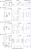
**Fig. 3. Effects of wildfire on occurrence or abundance were modified by fire-regime components.**
a–d, Mean standardized effect sizes (±95% CIs) for fire severity (a), and main effects or interactions with fire severity for fire frequency (number of fires 1979–2019) (b); inter-fire interval (years) preceding 2019–20 fires (c); unburnt vegetation within 2.5 km (d) (see Table 1 and Extended Data Fig. 6 for high, mid and low category boundaries). Orange row labels, low-severity fire; red row labels, high-severity fire; black row labels, main effect without severity interaction. Main effects are plotted when interactions had no statistical support (P > 0.1). Left panels (black), negative mean effect size (average effect size for all effects less than 0); central panels (grey), overall mean effect sizes (mean of all negative, zero and positive effects); right panels (blue), positive mean effect sizes (average effect size for all effects greater than 0). Error bars are symmetrical but truncated at −1 and 1. Vertical dotted line at 0 is a guide to when effects differ from zero. Numbers in black within panels above each result are the number of effects contributing to each mean effect (n). Boxplots of raw data are in light grey, indicating median, 25th and 75th percentiles, with whiskers 1.5× interquartile range. Numbers in light grey below a result at panel margins indicate whisker values (left and right panels) or box margins (centre panel) that exceeded x axis limits. Predicted values consider random effects so may not align with raw data. P values for plotted results are the omnibus two-tailed test. Test F statistics (from left to right) for fire severity: F(1,41) = 7.74; F(1,41) = 0.42; F(1,26) = 10.18; fire frequency: F(3,39) = 11.3; F(3,33) = 11.78; F(3,30) = 6.41; inter-fire interval: F(2,42) = 10.28; F(2,37) = 5.44; F(2,31) = 13.35; unburnt area: F(2,22) = 19.93; F(2,29) = 1.02; F(2,21) = 9.2.

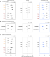
**Fig. 4. Pre-fire drought and tenure mediated the effects of wildfire.**
a–c, Mean standardized effects (±95% CI) of wildfire were modified by fire severity and its interaction with pre-fire drought (a), being in a protected area or not (b) and the proportion of protected area within 2.5 km (c). Orange row labels, low-severity fire; red row labels, high-severity fire; black row labels, main effect without severity interaction. Numbers in black within panels (n) are the number of effects contributing to each mean effect, and P values are for the plotted result. Panel layout and graphic features as in Fig. 3. Although the interaction of severity with drought for negative effects was weakly supported (a), the main effect was strongly supported (F(1,37) = 14.82, P < 0.001; Supplementary Table 1). Test F statistics (from left to right) for pre-fire drought: F(2,37) = 2.53; F(2,46) = 4.58; F(2,28) = 4.05; protected/unprotected area: F(1,44) = 3.33; F(1,46) = 0.62; F(1,31) = 8.54; extent of protected area: F(2,36) = 2.47; F(2,45) = 17.14; F(2,31) = 2.65.

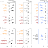
**Fig. 5. Wildfire impacts varied across taxa and ecosystems.**
a,b, Mean standardized effects (±95% CI) of wildfire on occurrence or abundance was modified by the interaction of fire severity with taxon (a) and ecosystem (b). Orange row labels, low severity fire; red row labels, high severity fire; black row labels, main effect without severity interaction. Numbers in black within panels are the number of effects contributing to each mean effect (n), and P values are for the plotted result. Panel layout and graphic features as in Fig. 3. Test F statistics (from left to right) for taxon: F(5,29) = 5.84; F(5,29) = 23.39; F(5,15) = 8.15; ecosystem: F(3,31) = 8.48; F(3,32) = 5.3; F(4,30) = 69.19.

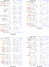
**Extended Data Fig. 1. Data extraction for calculating effect sizes.**
Flow diagram illustrating how the full dataset (1) was subdivided so that effect sizes could be calculated for each taxon within each project. Each row represents a record of taxon occurrence or abundance at an individual survey site within a project. (2) represents data treatment for covariates that varied at the taxon-within-project level (broad taxon, ecosystem type). (3) represents data treatment for covariates that differed between sites within projects (e.g. drought, inter-fire interval).

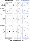
**Extended Data Fig. 2. How wildfire impacted occurrence or abundance was modified by study design, year, response, and region.**
Mean standardised effect sizes (±95% CI) for study design (a), year (b), and main effects or interactions with fire severity for response (c), and region (d). Graphic features as for Fig. 1. P values are for the plotted result and are the omnibus two-tailed test based on an F distribution. Test statistics (from left to right) for Study design: F(1,55) = 1.09, P = 0.302; F(1,61) = 1.26, P = 0.266; F(1,40) = 0.01, P = 0.917; Year: F(1,44) = 7.83, P = 0.008; F(1,47) = 15.57, P < 0.001; F(1,33) = 0.43, P = 0.519; Response: F(1,44) = 0.13, P = 0.724; F(1,47) = 0.7, P = 0.408; F(1,24) = 20.87, P < 0.001; Region: F(2,43) = 46.66, P < 0.001; F(2,46) = 25.96, P < 0.001; F(2,26) = 5.11, P = 0.013. Unburnt-burnt designs (Unb-burn, (a)) were used for all other analyses, so represent the overall effects of the 2019–20 fires without additional covariates. Before-after (Bef-after) survey designs produced a distribution of effect sizes that was shifted to the right with smaller negative and larger positive effects compared with unburnt-burnt designs, suggesting bias associated with the drought-breaking rains after the fires (a). In the second year after the fires there was a subtle reduction in mean negative effect sizes, hinting that recovery was beginning for some taxa that declined (b). Abundance (Abund) and occurrence (Occur) responses showed very similar effect sizes, with the only exception of higher positive effect sizes for occurrence data at high severity. The small number of effects in this group precludes further separate consideration of occurrence responses (c). The most striking regional effect was for weaker positive effects in the south, particularly at high severity (d). Fire conditions differed across regions. Our data suggest a weak trend towards stronger pre-fire drought in the south (Pearson’s correlation with latitude =−0.03, t = −2.5343, df = 6239, P = 0.01). Fires that drove the world’s most extreme pyrocumulonimbus event were all in our mid and southern regions, corresponding with larger contiguous areas of high severity fire. Remote sensing data indicate that the southern parts of the study region had slower rates of vegetation recovery than in the north. These differences in pre-fire conditions, fire behaviour, and recovery rates suggest that the level of disturbance and other stressors can constrain the response of taxa which would otherwise benefit from bushfires.

**Extended Data Fig. 3. Mean difference effect sizes (±95% CI).**
See previous figures for details. Panels match: top left; Fig. 3, top right; Fig. 4; bottom left; Fig. 5, bottom right Extended Data Fig. 2. Mean change effect size shown for Study design with before-after data, bottom right panel. P values are for the plotted result and are the omnibus two-tailed test based on an F distribution. Top left panel test statistics (from left to right): Fire severity: F(1,41) = 4.77, P = 0.035; F(1,41) = 0.7, P = 0.407; F(1,26) = 40.63, P < 0.001; Fire frequency: F(3,39) = 11.08, P < 0.001; F(3,33) = 2.68, P = 0.063; F(3,26) = 5.6, P = 0.004; Inter-fire interval: F(2,42) = 21.74, P < 0.001; F(2,37) = 13.77, P < 0.001; F(2,25) = 54.2, P < 0.001; Unburnt area: F(2,22) = 15.7, P < 0.001; F(2,29) = 43.89, P < 0.001; F(2,21) = 1.4, P = 0.268. Top right panel test statistics (from left to right): Pre-fire drought: F(2,37) = 4.06, P = 0.025; F(2,46) = 21.77, P < 0.001; F(2,28) = 13.48, P < 0.001; P.A. or Not: F(1,39) = 2.85, P = 0.1; F(1,46) = 2.01, P = 0.163; F(1,31) = 17.26, P < 0.001; P.A. area: F(2,36) = 12.09, P < 0.001; F(2,45) = 1.35, P = 0.271; F(2,25) = 5.32, P = 0.012. Bottom left panel test statistics (from left to right): Taxon: F(5,29) = 88.71, P < 0.001; F(5,29) = 22.98, P < 0.001; F(5,15) = 19.43, P < 0.001; Ecosystem: F(3,31) = 7.6, P = 0.001; F(3,32) = 69.68, P < 0.001; F(3,21) =2.58, P = 0.081. Bottom right panel test statistics (from left to right): Study design: F(1,55) = 0.18, P = 0.669; F(1,61) = 0.33, P = 0.569; F(1,40) = 2.56, P = 0.117; Year: F(1,39) = 5.35, P = 0.026; F(1,39) = 4.17, P = 0.048; F(1,33) = 1.72, P = 0.199; Response: F(1,39) = 14.86, P < 0.001; F(1,47) = 0.29, P = 0.594; F(1,24) = 21.87, P < 0.001; Region: F(2,37) = 16.53, P < 0.001; F(2,37) = 8.62, P = 0.001; F(2,26) = 19.61, P < 0.001.

**Extended Data Fig. 4. Mean difference or mean change effect sizes (±95% CI) calculated after outliers were removed.**
See previous figures for details. Panels match: top left; Fig. 3, top right; Fig. 4; bottom left; Fig. 5, bottom right Extended Data Fig. 2. P values are for the plotted result and are the omnibus two-tailed test based on an F distribution. Top left panel test statistics (from left to right): Fire severity: F(1,38) = 6.16, P = 0.018; F(1,38) = 1.8, P = 0.188; F(1,28) = 17.69, P < 0.001; Fire frequency: F(3,36) = 9.83, P < 0.001; F(3,37) = 2.58, P = 0.068; F(3,29) = 30.56, P < 0.001; Inter-fire interval: F(2,38) = 31.14, P < 0.001; F(2,34) = 11.31, P < 0.001; F(2,26) = 4.53, P = 0.021; Unburnt area: F(2,19) = 7.32, P = 0.004; F(2,26) = 54.6, P < 0.001; F(2,21) = 2.57, P = 0.101. Top right panel test statistics (from left to right): Pre-fire drought: F(2,34) = 2.77, P = 0.077; F(2,44) = 17.99, P < 0.001; F(2,27) = 5.05, P = 0.014; P.A. or Not: F(1,42) = 1.37, P = 0.248; F(1,43) = 2.2, P = 0.145; F(1,31) = 13.3, P = 0.001; P.A. area: F(2,31) = 12.15, P < 0.001; F(2,40) = 1.25, P = 0.299; F(2,27) = 5.44, P = 0.01. Bottom left panel test statistics (from left to right): Taxon: F(5,27) = 131.46, P < 0.001; F(5,27) = 19.34, P < 0.001; F(5,17) = 17.82, P < 0.001; Ecosystem: F(3,29) = 6.41, P = 0.002; F(3,30) = 9.74, P < 0.001; F(3,24) = 3.99, P = 0.019. Bottom right panel test statistics (from left to right): Study design: F(1,44) = 3.37, P = 0.073; F(1,56) = 0.51, P = 0.478; F(1,38) = 0.76, P = 0.389; Year: F(1,36) = 12.88, P = 0.001; F(1,36) = 9.9, P = 0.003; F(1,33) = 0.07, P = 0.796; Response: F(1,36) = 4.97, P = 0.032; F(1,45) = 0.25, P = 0.619; F(1,26) = 28.11, P < 0.001; Region: F(2,34) = 20.51, P < 0.001; F(2,34) = 5.26, P = 0.01; F(2,27) = 4.42, P = 0.022.

**Extended Data Fig. 5. Standardised effect sizes (±95% CI), with before-after designs retained in all analyses.**
See previous figures for details. Panels match: top left; Fig. 3, top right; Fig. 4; bottom left; Fig. 5, bottom right Extended Data Fig. 2. P values are for the plotted result and are the omnibus two-tailed test based on an F distribution. Top left panel test statistics (from left to right): Fire severity: F(1,50) = 8.49, P = 0.005; F(1,54) = 0.39, P = 0.533; F(1,35) = 11.54, P = 0.002; Fire frequency: F(3,49) = 12.21, P < 0.001; F(3,46) = 4.49, P = 0.008; F(3,39) = 8.58, P < 0.001; Inter-fire interval: F(2,53) = 9.36, P < 0.001; F(2,59) = 14.16, P < 0.001; F(2,40) = 13.97, P < 0.001; Unburnt area: F(2,31) = 18.01, P < 0.001; F(2,43) = 1.06, P = 0.356; F(2,30) = 5.98, P = 0.007. Top right panel test statistics (from left to right): Pre-fire drought: F(2,46) = 2.96, P = 0.062; F(2,60) = 4.07, P = 0.022; F(2,37) = 3.92, P = 0.029; P.A. or Not: F(1,55) = 2.02, P = 0.161; F(1,60) = 0.95, P = 0.334; F(1,40) = 3.82, P = 0.058; P.A. area: F(2,54) = 0.62, P = 0.54; F(2,59) = 18.08, P < 0.001; F(2,40) = 2.19, P = 0.126. Bottom left panel test statistics (from left to right): Taxon: F(5,38) = 6.85, P < 0.001; F(5,42) = 23.4, P < 0.001; F(5,24) = 10.32, P < 0.001; Ecosystem: F(3,39) = 7.89, P < 0.001; F(3,42) = 2.98, P = 0.042; F(4,37) = 44.21, P < 0.001. Bottom right panel test statistics (from left to right): Study design: F(1,55) = 1.09, P = 0.302; F(1,61) = 1.26, P = 0.266; F(1,40) = 0.01, P = 0.917; Year: F(1,55) = 5.82, P = 0.019; F(1,61) = 15.46, P < 0.001; F(1,42) = 0.17, P = 0.682; Response: F(1,55) = 0.32, P = 0.576; F(1,61) = 2.09, P = 0.154; F(1,33) = 5.98, P = 0.02; Region: F(2,54) = 28.4, P < 0.001; F(2,60) = 27.24, P < 0.001; F(2,35) = 5.26, P = 0.01.

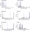
**Extended Data Fig. 6. Distribution of covariate data.**
Blue vertical lines indicate cut points for categories.

See this image and copyright information in PMC

References

1. Feng, X. et al. How deregulation, drought and increasing fire impact Amazonian biodiversity. Nature597, 516–521 (2021). - PubMed
1. Kelly, L. T. et al. Fire and biodiversity in the Anthropocene. Science370, eabb0355 (2020). - PubMed
1. Peterson, D. A. et al. Australia’s Black Summer pyrocumulonimbus super outbreak reveals potential for increasingly extreme stratospheric smoke events. npj Clim. Atmos. Sci.4, 38 (2021).
1. Collins, L. et al. The 2019/2020 mega-fires exposed Australian ecosystems to an unprecedented extent of high-severity fire. Environ. Res. Lett.16, 044029 (2021).
1. Penman, T. D., Clarke, H., Gibson, R. K., Collins, L. & Nolan, R. H. in Australia’s Megafires: Biodiversity Impacts and Lessons From 2019–2020 (eds Rumpff, L. et al.) 42–59 (CSIRO, 2023).

MeSH terms

Actions
Actions
Actions
Actions
Actions
Actions
Actions
Actions
Actions
Actions
Actions
Actions
Actions
Actions
Actions

LinkOut - more resources

Full Text Sources
- Nature Publishing Group
- PubMed Central
Medical
- MedlinePlus Health Information
Miscellaneous
- NCI CPTAC Assay Portal

Save citation to file

Email citation

Add to Collections

Add to My Bibliography

Your saved search

Create a file for external citation management software

Your RSS Feed

Biodiversity impacts of the 2019-2020 Australian megafires

Affiliations

Biodiversity impacts of the 2019-2020 Australian megafires

Authors

Affiliations

Abstract

Conflict of interest statement

Figures

References

MeSH terms

LinkOut - more resources

Full Text Sources

Medical

Miscellaneous