Optimal Operation of Cryogenic Calorimeters Through Deep Reinforcement Learning

Abstract

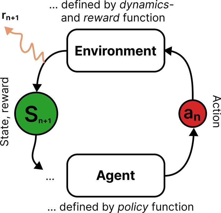
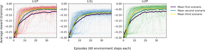
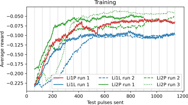
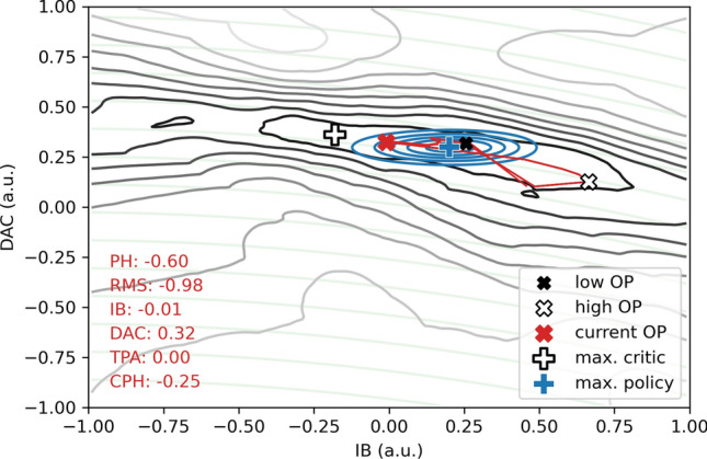
Cryogenic phonon detectors with transition-edge sensors achieve the best sensitivity to sub-GeV/c $_{}^2$ dark matter interactions with nuclei in current direct detection experiments. In such devices, the temperature of the thermometer and the bias current in its readout circuit need careful optimization to achieve optimal detector performance. This task is not trivial and is typically done manually by an expert. In our work, we automated the procedure with reinforcement learning in two settings. First, we trained on a simulation of the response of three Cryogenic Rare Event Search with Superconducting Thermometers (CRESST) detectors used as a virtual reinforcement learning environment. Second, we trained live on the same detectors operated in the CRESST underground setup. In both cases, we were able to optimize a standard detector as fast and with comparable results as human experts. Our method enables the tuning of large-scale cryogenic detector setups with minimal manual interventions.

Keywords: Cryogenic calorimeter; Dark matter; Reinforcement learning; Transition-edge sensor.

Fig. 1

Schematic drawing of the detector environment. The circuits are schematical visualizations and not complete electrical and thermal circuits. (center) The detector can be described as an electrothermal system, where the readout and heater electronics and the temperatures in the crystal and sensor interact with each other. Visualizations of the thermal system are in blue and of the electrical system in black. The readout circuit of the TES (central in the figure) and the heater circuit (lower center) are electrically separated. (right) The recorded observable from particle recoils is a pulse-shaped voltage signal (orange) in superposition with sensor noise (black). Features to quantify the quality of the detector response can be extracted from the pulse shape, using the pulse height (PH) and root-mean-square (RMS) values. (left) A policy neural network is trained with reinforcement learning (RL) to choose optimal control parameters based on the state of the system. Optimal control parameters maximize the return, a target function that is closely related to the signal-to-noise ratio (SNR). A maximal return realizes a trade-off between low-noise amplitude, linear range of the detector, and stable measurement conditions. See text in “Modeling the Detector Response and Noise” and “Optimizing the Sensitivity” sections for details

Fig. 2

The mechanics of RL: an agent follows a policy function to interact with an environment. The environment, defined by its dynamics and reward function, responds to the agent’s actions with a reward and observable state (Figure adapted from Ref. [6])

Fig. 3

Simulation and measurement of a 5.95 keV X-ray event induced by a calibration source in the Li1P detector. (upper left) The OP (black/blue lines) within the simulated transition curve of the TES (light red line). A measurement of the transition curve is shown for comparison (grey dots). (upper right) The voltage pulse induced in the simulated SQUID amplifier without noise (red) and overlayed with noise generated from the simulated NPS (black). A measured voltage pulse is shown for comparison (grey dashed). (lower part) The simulated NPS (black) has individual noise contributions (colored). The 1/f, excess Johnson, and EM interference noise components were adjusted to fit the measured NPS (grey dashed)

Fig. 4

The average rewards per episode during training for all 105 versions of the three detectors Li1P (red, left), Li1L (blue, center), and Li2P (green, right). The thick lines are the mean values of all curves corresponding to the first/second/third scenario (violet/turquoise/yellow). The mean values rise close to the apex of the curves after 15 to 20 episodes. The second and third scenarios reach convergence significantly faster than the first. During the first 5 to 10 episodes, only little return is collected. The distribution of curves is clearly not normally distributed around the mean value, which is due to the different hyperparameter settings in the training of the individual detector versions

Fig. 5

Histogram of the average reward achieved during inference trajectories with the trained agents for the 105 versions of Li1P (red, top), Li1L (blue, center), and Li2P (green, bottom) each. Rewards from versions with opportune choices of hyperparameters cluster around a benchmark value (black line), achieved by a human expert. The suboptimal versions appear at lower reward values in the histogram. The results of Li1L surpass the benchmark value, since higher pulses saturate stronger in this detector, which can be accounted for with the machine learning method

Fig. 6

Schematic visualization of the implemented setup to optimize CRESST detector control. (right side) The detectors are operated in a cryostat and read out by a DAQ system. The parameters of recorded test pulses are sent via a Message Queues Telemetry Transport (MQTT) [21] broker to a client, as state. (left side) The client calculates the reward from the state, stores the data in an experience replay buffer, and responds to the DAQ system with new control parameters. An independent process trains the AC agent on the buffer. This is a symbolic visualization, the algorithm we are using is the SAC algorithm

Fig. 7

Average rewards per test pulse sent during the live training on the CRESST setup, smoothed with a moving average of 60 test pulses. Results from six runs with different training settings are shown for Li1P (red), Li1L (blue, blue dashed), and Li2P (green, green dashed, green dotted). For this comparison, we re-calculated the rewards after training with Eq. (2), while during training for some of the runs, the unweighted reward function Eq. (1) was used

Fig. 8

Visualization of the cyclic adjustment of the control parameters during an inference trajectory on Li1L, run 2. The ascending trajectory of injected test pulses is visualized in the circle in the anti-clockwise direction. The voltage traces of the observed pulses (black) are normalized to a fixed voltage interval. The pulses are normalized to the applied bias current, leading to smaller pulses and noise for higher IB. The TPA values (bold) and measurement time since the start of the test pulse trajectory are written next to the voltage traces. The polar plot includes the IB and DAC values that were set while the corresponding pulse was recorded. Their values are normalized to the interval − 1 to 1 (see Appendix E for normalization ranges). The polar axis starts at − 0.5, and the distance between the grey rings corresponds to an increase of 0.5. Three OPs are marked with black, red, and white crosses, corresponding to OPs that were chosen for low, intermediate, and high TPA values

Fig. 9

Histogram of the average reward obtained during inference trajectories with the trained agents on the real-world versions of Li1P (red, top), Li1L (blue, center), and Li2P (green, bottom) each. The rewards obtained in the simulation (grey, dotted histogram) and the human-optimized benchmark value (black line) are shown for comparison. The obtained rewards are worse than the benchmark value but correspond to our expectations from the simulation. For a discussion of the achievable optimality, see also Fig. 10

Fig. 10

Visualization of the Gaussian policy probability distribution (blue) and the critic function (grey-black) over the two-dimensional action space, for a fixed “current” state (red text, lower left) and Li1L run 2. The maximum of the critic function is marked with a white plus. The current control parameters are marked with a red cross, that of OPs that were chosen by the agent for high/low TPA values with a white/black cross. These crosses correspond to the OPs marked with similar crosses in Fig. 8. The trajectory of actions that are chosen by the agent in inference is drawn with a red line, partially covered by the blue policy function. We can clearly see a mismatch between the actions preferred by the policy function and the maximum of the critic function. The reason for this mismatch is discussed in the text and in Appendix G. The expected lines of constant heating caused by the DAC through the heating resistor and the IB through Joule heating are shown in the background (light, transparent green). As expected, the island of actions that the critic prefers stretches along the constant heating lines and corresponds to a fixed resistance of the TES. The state values are normalized to the interval − 1 to 1. The original value ranges are written in Table 2

Fig. 11

Average reward during all training episodes of the different versions of the virtual detectors, grouped into violins for each scenario (violet, turquoise, yellow) and setting of the hyperparameters learning rate (lr), batch size (bs), $\gamma$ and gradient steps (gs). Each violin includes five versions of Li1P, Li1L, and Li2P each, sampled and trained with individual random seeds. The red bars indicate the mean values of the violins and their thickness the density of the represented return distribution. The dotted horizontal lines indicate the mean values of the collected returns of the first (lowest), second, and third (highest) scenarios of detector versions. The dotted vertical lines separate the violins with different hyperparameter settings. The values for the hyperparameters are written in the ticks on the abscissa

Fig. 12

Movement of a SAC agent in a two-dimensional toy box environment. The goal of the agent is to jump close to the cyclically changing target lines (black dashed). The paths taken by an agent in inference trajectories are drawn with colored lines, for different magnitudes of the jump regularization parameter $\omega$

Fig. 13

Toy environment of an agent that climbs a mountain. The reward function (black) has the shape of a side view of the mountain that ends in a cliff on one side. The critic function (green) learns the shape of the reward function sufficiently well. The policy function (red) learns to overlap with the mountain, instead of placing its expected value on top of the mountain (see text for details). To keep all actions in the interval between − 1 and 1, the actions sampled from the Gaussian are again input to a hyperbolic tangent function in the SAC algorithm. This leads to a deviation between the mean, the median, and the mode of the resulting probability distribution. We show by comparing the expected/mean value of the policy (red dashed) with its median (grey) and its modus (peak of the red Gaussian) that this effect does not play a significant role in our experiment

Fig. 14

Return per episode for Li1P (red), Li1L (blue) and Li2P (green) adjusted to two TES. The thick line represents the mean of five trained versions of the detectors, sampled with different random seeds. The shaded region shows the upper and lower standard deviations. We show benchmarks (dashed lines) for all three detectors. These benchmarks were calculated by taking the average reward in the last episode of the training for all versions of the single-TES detectors that were trained in “Operation in a Virtual Environment” section, and multiplying it by two. The benchmark is reached by Li1P and Li2P, but not by Li1L

References

1. Irwin K, Hilton G (2005) Transition-edge sensors. In: Enss C (ed) Cryogenic particle detection. Springer, Berlin, pp 63–150. 10.1007/10933596_3 (ISBN 978-3-540-31478-3)
1. Abdelhameed AH et al (2019) First results from the cresst-iii low-mass dark matter program. Phys Rev D 100:102002. 10.1103/PhysRevD.100.102002
1. Cresst homepage. https://cresst-experiment.org/. Accessed 10 Apr 2024.
1. Angloher G et al (2023) Results on sub-gev dark matter from a 10 ev threshold cresst-iii silicon detector. Phys Rev D 107:122003. 10.1103/PhysRevD.107.122003
1. Billard J et al (2022) Direct detection of dark matter—APPEC committee report*. Rep Progr Phys 85(5):056201. 10.1088/1361-6633/ac5754 - PubMed
LinkOut - more resources