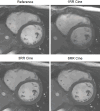
Accelerated Cardiac MRI with Deep Learning-based Image Reconstruction for Cine Imaging

Abstract

Purpose To assess the influence of deep learning (DL)-based image reconstruction on acquisition time, volumetric results, and image quality of cine sequences in cardiac MRI. Materials and Methods This prospective study (performed from January 2023 to March 2023) included 55 healthy volunteers who underwent a noncontrast cardiac MRI examination at 1.5 T. Short-axis stack DL cine sequences of the left ventricle (LV) were performed over one (1RR), three (3RR), and six cardiac (6RR) cycles and compared with a standard cine sequence (without DL, performed over 10-12 cardiac cycles) in regard to acquisition time, subjective image quality, edge sharpness, and volumetric results. Results Total acquisition time (median) for a short-axis stack was 47 seconds for the 1RR cine, 108 seconds for 3RR cine, 184 seconds for 6RR cine, and 227 seconds for the standard sequence. Volumetric results showed no difference for the conventional cine (median LV ejection fraction [EF] 63%), 6RR cine (median LVEF, 62%), and 3RR cine (median LVEF, 61%). The 1RR cine sequence significantly underestimated EF (57%) because of a different segmentation of the papillary muscles. Subjective image quality (P = .37) and edge sharpness (P = .06) of the three-heartbeat DL cine did not differ from the reference standard, while both metrics were lower for single-heartbeat DL cine and higher for six-heartbeat DL cine. Conclusion For DL-based cine sequences, acquisition over three cardiac cycles appears to be the optimal compromise, with no evidence of differences in image quality, edge sharpness, and volumetric results, but with a greater than 50% reduced acquisition time compared with the reference sequence. Keywords: MR Imaging, Cardiac, Heart, Technical Aspects, Cardiac MRI, Deep Learning, Clinical Imaging, Accelerated Imaging Supplemental material is available for this article. © RSNA, 2024.

Keywords: Accelerated Imaging; Cardiac; Cardiac MRI; Clinical Imaging; Deep Learning; Heart; MR Imaging; Technical Aspects.

Figure 1:

Visualization of acquisition schemes. For a cardiac MRI cine acquisition, the k-space is divided into segments (colored boxes), and each segment needs to be sampled in all cardiac phases, as seen in the lower part of the figure. For a standard sequence (right), the k-space is sampled uniformly, resulting in the segments having equal size. For variable density sampling (left), the outer k-space segments have fewer points, and hence, a larger segment can be acquired within the same time. The segment size is adjusted to the sampling density, resulting in fewer segments overall and hence, an accelerated acquisition.

Figure 2:

Schematic representation of deep learning–based image reconstruction. An unrolled neural network is used in DLCine to reconstruct cine images from the undersampled k-space data. The network includes multiple iterations (unrolled blocks), with each block containing a data consistency module and a neural network–based regularizer.

Figure 3:

Quantification of edge sharpness. (Top) Axial noncontrast cardiac cine MR images for each sequence type, with red profile line. (Bottom) Graphs show the normalized intensity profile and regression line over the blood to myocardium transition for edge sharpness determination. C_norm = normalized intensity profile, C̃_norm = intensity profile used for edge sharpness calculation, C^'_norm = first derivative of C_norm' f(s_i) = linear regression of intensity profile used for edge sharpness calculation, Len_Profile = length of profile line from blood pool to myocardium, 1RR = one cardiac cycle cine sequence, Ref = reference sequence, s = distance, 6RR = six cardiac cycles cine sequence, 3RR = three cardiac cycles cine sequence.

Figure 4:

Image examples in a healthy volunteer (31-year-old male). Axial noncontrast cardiac MR images from reference cine sequence, one cardiac cycle (1RR) cine, three cardiac cycles (3RR) cine, and six cardiac cycles (6RR) cine are shown. Cine video files from this case are available as Movies 1–4.

Figure 5:

Volumetric results. Box plots show the results for LV EDV, LV ESV, LV SV, and LV mass indexed to body surface area for reference, one cardiac cycle (1RR), three cardiac cycles (3RR), and six cardiac cycles (6RR) cine sequences. Boxes represent the 5%–95% interval. The line inside each box indicates the median. Whiskers indicate the minimum and maximum values. LV EDV = left ventricular end-diastolic volume, LV ESV = left ventricular end-systolic volume, LV SV = left ventricular stroke volume.

References

-
- Currie G , Hawk KE , Rohren E , Vial A , Klein R . Machine learning and deep learning in medical imaging: intelligent imaging . J Med Imaging Radiat Sci 2019. ; 50 ( 4 ): 477 – 487 . - PubMed
- Orii M , Sone M , Osaki T , et al. . Reliability of respiratory-gated real-time two-dimensional cine incorporating deep learning reconstruction for the assessment of ventricular function in an adult population . Int J Cardiovasc Imaging 2023. ; 39 ( 5 ): 1001 – 1011 . - PubMed
MeSH terms
LinkOut - more resources
Full Text Sources