Scalable, data-assimilated models predict large-scale shoreline response to waves and sea-level rise

Abstract

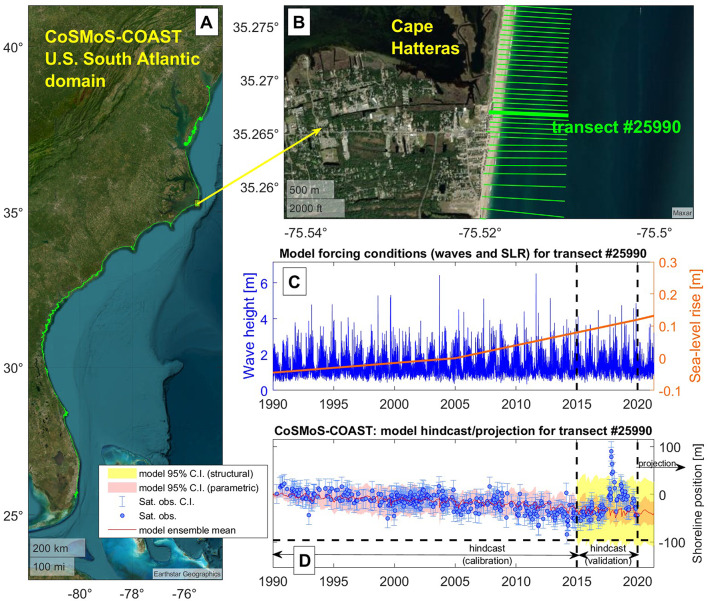
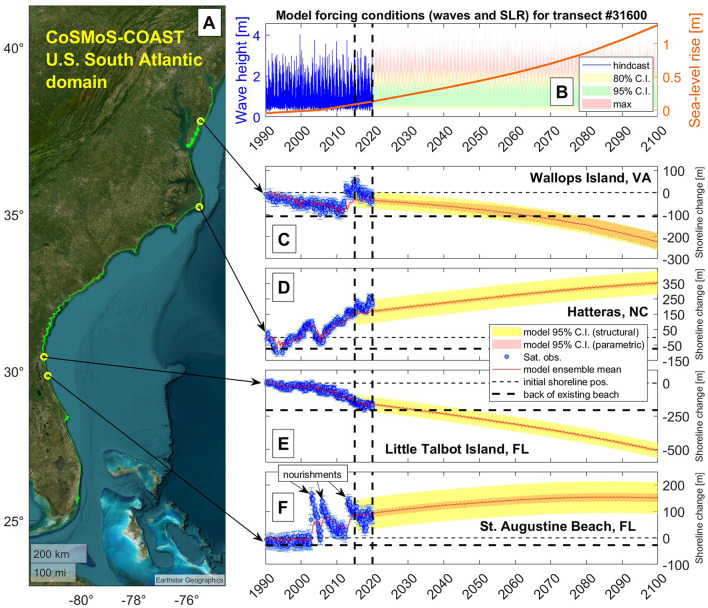
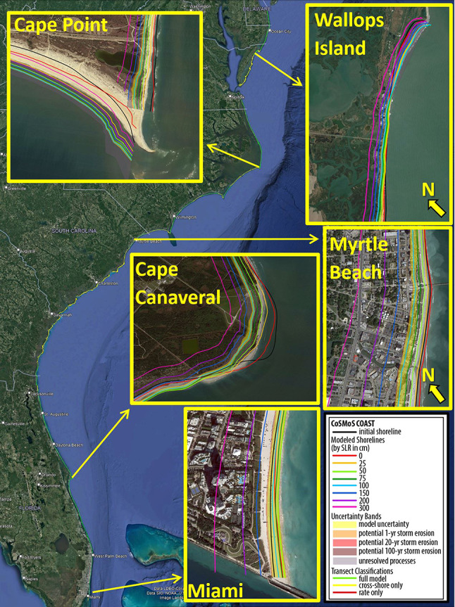
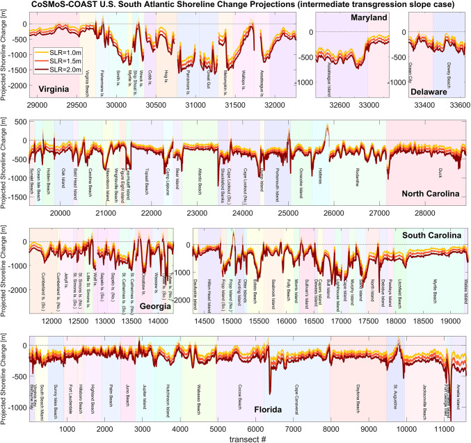
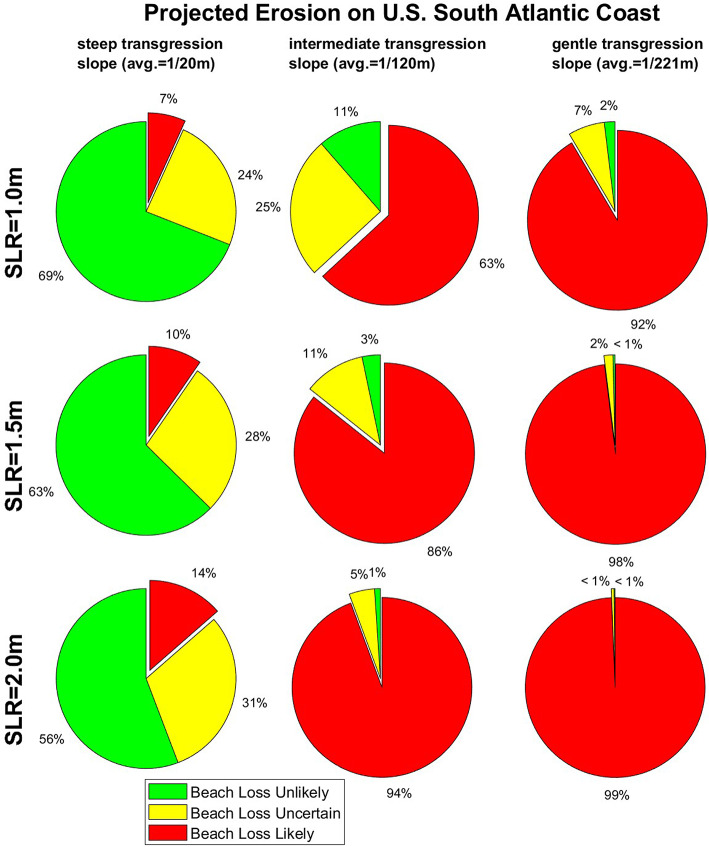
Coastal change is a complex combination of multi-scale processes (e.g., wave-driven cross-shore and longshore transport; dune, bluff, and cliff erosion; overwash; fluvial and inlet sediment supply; and sea-level-driven recession). Historical sea-level-driven coastal recession on open ocean coasts is often outpaced by wave-driven change. However, future sea-level-driven coastal recession is expected to increase significantly in tandem with accelerating rates of global sea-level rise. Few models of coastal sediment transport can resolve the multitude of coastal-change processes at a given beach, and fewer still are computationally efficient enough to achieve large-scale, long-term simulations, while accounting for historical behavior and uncertainties in future climate. Here, we show that a scalable, data-assimilated shoreline-change model can achieve realistic simulations of long-term coastal change and uncertainty across large coastal regions. As part of the modeling case study of the U.S. South Atlantic Coast (Miami, Florida to Delaware Bay) presented here, we apply historical, satellite-derived observations of shoreline position combined with daily hindcasted and projected wave and sea-level conditions to estimate long-term coastal change by 2100. We find that 63 to 94% of the shorelines on the U.S. South Atlantic Coast are projected to retreat past the present-day extent of sandy beach under 1.0 to 2.0 m of sea-level rise, respectively, without large-scale interventions.

Fig. 1

An example of calibration and validation of CoSMoS-COAST using historical satellite-derived shoreline data. The figure shows the extent of the CoSMoS-COAST U.S. South Atlantic Coast model transects (panel A—in green) with a zoomed in section of Cape Hatteras, North Carolina (panel B), which shows a close-up of the 50 m transect spacing (green lines). Panel C shows hindcasted and projected wave (blue line) and sea-level rise conditions (orange line) applied to the model at transect #25990 (i.e., the thick green line in panel B). Panel D shows the modeled shoreline position (red line) and its parametric uncertainty (pink bands), which are calibrated (from 1990–2015) with satellite-derived shoreline observations (blue circles) and their confidence intervals (blue ‘whiskers’). Later in the simulation, during the model “hindcast (validation)” period (2015–2020), data assimilation is turned off, and the calibrated model is compared to satellite-derived shoreline observations (blue circles) to assess the model’s structural uncertainty (, where is the model root-mean square error (RMSE) calculated using Eq. (2) and is shown in yellow confidence bands), which is propagated forward with a constant width during the model ‘projection period’ (2020–2100). Note that anomalies in shoreline position during the “hindcast (validation)” period, e.g., the accretion spike in 2017–2018 in panel D (caused by a beach nourishment), generally increase the model’s structural uncertainty (yellow bands) relative to the parametric uncertainty (pink bands). (Basemap from Matlab/Earthstar Geographics/Maxar).

Fig. 2

Examples of long-term simulations of shoreline change with CoSMoS-COAST until 2100. The extent of the U.S. South Atlantic Coast model domain (panel A—transects in green) with model results at Wallops Island, Va., Hatteras, N.C., Little Talbot Island, Fla., and St. Augustine, Fla. (transect # 31600, 25880, 11150, and 9805, respectively). Panel B shows hindcasted (blue line) and projected (ensemble) wave (green, yellow, and red confidence bands) and sea-level rise conditions (orange line) applied to the model at transect #31600 (Wallops Island, Va.). Panels C, D, E, and F show the long-term modeled shoreline position (red line) and its parametric (pink band) and structural uncertainty (yellow band). The parametric uncertainty (pink band) is calibrated (from 1990–2015) with satellite-derived shoreline observations (blue circles) and their confidence intervals (blue ‘whiskers’). Later in the simulation, the model is validated (during the period 2015–2020) to assess the model’s structural uncertainty (, where is the model root-mean square error (RMSE) calculated using Eq. (2) and is shown in yellow confidence bands), which is propagated forward with a constant width during the model ‘projection period’ (2020–2100). Note that anomalies in shoreline position due to beach nourishments (e.g., panel F), generally mask naturally occurring erosion trends and thus increase the tendency for the model to infer/assimilate accretion trends from historical observations. (Basemap from Matlab/Earthstar Geographics).

Fig. 3

Examples of shoreline modeling projections for ~ 1,850 km of coastline in on the U.S. South Atlantic Coast (full data available online at [SC, NC], [FL, GA, VA, MD, DE]), which are shown here for the “unimpeded” and “continued accretion” model case scenarios and the intermediate transgression slope (described in “Methods” section and shown in S8, respectively). The projections represent the shoreline position in 2100 with various projections of sea-level rise. The yellow bands represent the projected shoreline position and (parametric) uncertainty, and the orange/red bands (shown only for the 1.0 m sea-level scenario for clarity) represent the potential storm-driven erosion uncertainty determined following Vitousek et al.. (Basemap from Google Earth).

Fig. 4

Model-projected shoreline positions in 2100 (relative to the initial shoreline position obtained from satellite-derived shoreline observations ca. 1990) versus transect number (numbered consecutively from south to north) for the intermediate transgression-slope scenario (see S10 and S11 for plots of the high and low transgression slope scenarios, respectively). Note that each panel represents a different state on the U.S. South Atlantic Coast, and each panel has different limits on the y-axis. The figure illustrates the shoreline-change simulations due to sea-level rise (SLR) projections of 1.0, 1.5, and 2.0 m by 2100 in yellow, orange, and red colors, respectively, under the “unimpeded” and “continued accretion” model cases (see “Methods” section). Sections of the yellow, orange, and red lines in this figure are plotted as either thin or thick lines, which indicate that the projected shoreline position is either seaward or landward of the existing end of the sandy beach, respectively. Hence, the thin line segments indicate portions of the coastline where sandy beaches are still present in 2100, whereas thick line segments indicate where sandy beaches have become lost in 2100, while assuming a static back beach line.

Fig. 5

Projected beach loss on the U.S. South Atlantic Coast (Florida to Delaware) as a function of sea-level rise (i.e., different rows) and transgression-slope case (i.e., different columns), and assuming the “impeded” model case, i.e., hardened, unyielding back-beach infrastructure and vegetation, which represent lower-bounded projections of potential beach change. The green, yellow, and red sections of the pie charts indicate the percentage of coastline with low, intermediate, and high likelihood of beach loss (i.e., where the modeled shoreline recedes landward into existing beach boundaries of urban infrastructure or back-beach vegetation). Note that the prevalence of beach loss is highly sensitive to the transgression slopes applied to the model (which are spatially variable and are shown in S8).

References

1. Hapke, C. J., Plant, N. G., Henderson, R. E., Schwab, W. C. & Nelson, T. R. Decoupling processes and scales of shoreline morphodynamics. Mar. Geol.381, 42–53 (2016).
1. Larson, M. & Kraus, N. C. Prediction of cross-shore sediment transport at different spatial and temporal scales. Mar. Geol.126(1–4), 111–127 (1995).
1. Murray, A. B. Reducing model complexity for explanation and prediction. Geomorphology90(3–4), 178–191 (2007).
1. Vitousek, S., Barnard, P. L. & Limber, P. Can beaches survive climate change?. J. Geophys. Res. Earth Surf.122(4), 1060–1067 (2017).
1. Hoagland, S. W. et al. Advances in morphodynamic modeling of coastal barriers: A review. J. Waterw. Port Coast. Ocean Eng.149(5), 03123001 (2023).
LinkOut - more resources