A High-Fidelity Computational Model for Predicting Blood Cell Trafficking and 3D Capillary Hemodynamics in Retinal Microvascular Networks

Abstract

Purpose: To present a first principle-based, high-fidelity computational model for predicting full three-dimensional (3D) and time-resolved retinal microvascular hemodynamics taking into consideration the flow and deformation of individual blood cells.

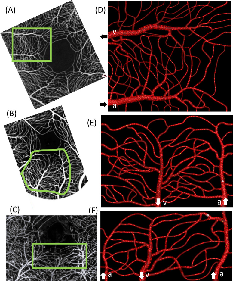
Methods: The computational model is a 3D fluid-structure interaction model based on combined finite volume/finite element/immersed-boundary methods. Three in silico microvascular networks are built from high-resolution in vivo motion contrast images of the superficial capillary plexus in the parafoveal region of the human retina. The maximum tissue area represented in the model is approximately 500 × 500 µm2, and vessel lumen diameters ranged from 5.5 to 25 µm covering capillaries, arterioles, and venules. Blood is modeled as a suspension of individual blood cells, namely, erythrocytes (RBC), leukocytes (WBC), and platelets in plasma. An accurate and detailed biophysical modeling of each blood cell and their flow-induced deformation is considered. A physiological, pulsatile boundary condition corresponding to an average cardiac cycle of 0.9 second is used.

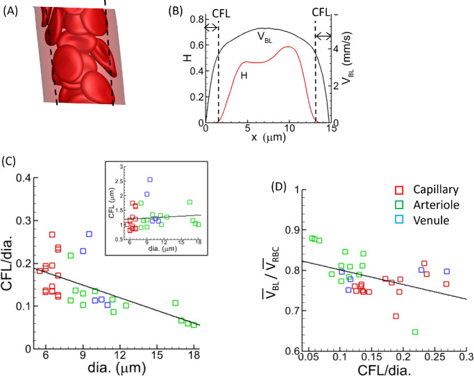
Results: Detailed quantitative data and analysis of 3D retinal microvascular hemodynamics are presented, and their relationship to RBC flow dynamics is illustrated. Blood velocity is shown to have temporal oscillations superimposed on the background pulsatile variation, which arise because of the way RBCs partition at vascular junctions, causing repeated clogging and unclogging of vessels. Temporal variations in RBC velocity and hematocrit are anti-correlated in a given vessel, but their time-averaged distributions are positively correlated across the network. Whole blood velocity is 65% to 85% of RBC velocity, with the discrepancy related to the formation of an RBC-free region, adjacent to the vascular endothelium and typically 0.8 to 1.8 µm thick. The 3D velocity and RBC concentration profiles are shown to be oppositely skewed with respect to each other, because of the way that RBCs "hug" the apex of each bifurcation. RBC deformation is predicted to have biphasic behavior with respect to vessel diameter, with minimal cell length for vessels approximately 7 µm in diameter. The wall shear stress (WSS) exhibits a strongly 3D distribution with local regions of high value and gradient spanning a range of 10 to 80 dyn/cm2. WSS is highest where there is faster flow, greater curvature of the vessel wall, capillary bifurcations, and at locations of RBC crowding and associated thinning of the cell-free layer.

Conclusions: This study highlights the usefulness of high-fidelity cell-resolved modeling to obtain accurate and detailed 3D, time-resolved retinal hemodynamic parameters that are not readily available through noninvasive imaging approaches. The results presented are expected to complement and enhance the interpretation of in vivo data, as well as open new avenues to study retinal hemodynamics in health and disease.

Figure 1.

(A–C) In vivo images of the human parafoveal microvascular networks obtained from references 4 and 30 (with permission). Green box indicates the tissue area modeled. Corresponding in silico models and RBC distribution as predicted by our model at one time instant are shown in D–F. Arrows indicate flow directions at inlets and outlets, and a and v indicate arterioles and venules, respectively. Animations of predicted RBC flow in the modeled in silico vasculatures are given in Supplementary Materials.

Figure 2.

(A) Triangular mesh on vessel surface in a small segment of a microvasculature in silico. (B–D) Resting shapes and sizes of a RBC, a mononucleated WBC, and a platelet. An example mesh on the RBC surface is shown. Biophysical properties of the cells used in the model are also noted. For WBCs and platelets, shear and area dilation moduli are taken 10 times higher since they are much less deformable than RBCs. (E) Pulsatile profile specified at an inlet vessel. (F–I) Different RBC flow patterns as predicted by the model are shown in a few vessels. (F) Single-file RBC flow in one capillary, (H) double file and zig-zag patterns, and (G, I) multi-file flow in larger vessels. RBCs are shown in red, platelets in yellow, and WBC in gray.

Figure 3.

Comparison of the model predictions against in vivo data reported for human retinal microcirculation. (A) Pulsatile profile of the RBC velocity as predicted by the model (continuous curves in color) in a few capillary vessels compared against Bedggood & Metha (dash black curve). (B) Predicted pulsatility index and minimum RBC velocity V_min compared against Neriyanuri et al. and Gu et al.. (C) RBC lineal density predicted against Gu et al.

Figure 4.

Quantification of RBC velocity and whole blood velocity differences. (A) Pulsatile profiles of RBC velocity (dash) and whole blood velocity (solid) in one vessel. (B) Time-averaged RBC (${\overline{V}}_{RBC}$, filled symbols) and whole blood (${\overline{V}}_{BL}$, open symbols) velocity versus vessel diameter in all vessels of a simulated vascular network. (C) The ratio ${\overline{V}}_{BL}/{\overline{V}}_{RBC}$ versus vessel diameter. For B and C, red, green, and blue symbols indicate capillaries, arterioles, and venules, respectively.

Figure 5.

(A) A snapshot of RBC distribution in a vessel segment in a simulated vasculature. (B) Radial distribution of blood velocity (right axis, black curve) and RBC concentration H (left axis, red curve) in the vessel. CFL is marked in A and B by dashed lines. (C) Ratio of CFL thickness to vessel diameter versus vessel diameter for all vessels in one vasculature (R² = 0.38, P < 0.001). Inset shows CFL versus vessel diameter with no significance dependence. (D) The ratio of blood velocity to RBC velocity in each vessel versus CFL thickness to diameter ratio (R² = 0.18, P = 0.013). For C and D, red, green, and blue symbols represent capillaries, arterioles and venules, respectively.

Figure 6.

Predicted RBC lengths in a network as a function of vessel diameter. Green delta represents average cell length over one pulsatile period. Red squares and black circles represent cell lengths over a 0.2-second window around the peak and low flow rates, respectively. Also shown are visualizations in a few vessel segments illustrating the role of confinement, and different flow patterns on RBC deformation.

Figure 7.

Quantifying time-dependent fluctuations. (A) RBC velocity versus time shown in several vessels appears as superposition of a background pulsatile profile (black dashed curve) and fluctuations. (B) Hematocrit versus time shows similar fluctuations, but no pulsatile profile. (C) MAD of RBC (V′_RBC, filled symbols) and whole blood (V′_BL, open symbols) velocity fluctuations w.r.t background pulsatile profile. (D) MAD for hematocrit (H′). In C and D, different colors indicate capillaries, arterioles, and venules as noted.

Figure 8.

RBC dynamics causes fluctuations in velocity and hematocrit. (A–D) Time history of RBC velocity (left axis, black solid curve) and hematocrit (right axis, red dash curves) in a few interconnected vessels over one cardiac cycle. The vessels are shown in E and F and identified by numbers 42–44, 46. (E, F) RBC distributions at two instances (also marked in A–D by colored vertical lines). Arrows give flow direction. (G) Cross-correlation between RBC velocity and blood velocity (red squares) and between RBC velocity and hematocrit (black circles) in each vessel.

Figure 9.

(A, B) Average hematocrit in each vessel plotted against the average whole blood velocity and vessel diameter, respectively. R² = 0.31, P < 0.001 for A, and R² = 0.15, P = 0.002 for B. Red, green, and blue symbols correspond to capillaries, arterioles, and venules, respectively. (C, D) Maps of hematocrit and whole blood velocity (mm/s), respectively. Arrows indicate vessels near the FAZ with low velocity and hematocrit.

Figure 10.

(A) An instantaneous image showing RBCs flow through a bifurcation. RBCs flow along the side of a daughter vessel that is closer to the apex of a bifurcation. (B) Resulting blood velocity and hematocrit distributions are skewed to opposite sides in the daughter vessels as marked 1 and 2. (C, D) The 2D profiles of velocity (black) and hematocrit (red) along the vessel diameter for 1 and 2, respectively. (E) Velocity skewness S_V versus hematocrit skewness S_H at the beginning and (F) end of a vessel, respectively. Red, green, and blue symbols represent capillaries, arterioles, and venules, respectively.

Figure 11.

(A, B) The 3D distribution of WSS in the full (RBC included) model and using cell-free Newtonian fluid, respectively. Thick arrows indicate focal nature of WSS; circles indicate high WSS regions near the bifurcations; thin arrows indicate WSS variation in high curvature regions. (C, D ) Close-up view of the WSS and its gradient at a bifurcation and RBC lingering causing such high values. (E, F) The WSS distribution in a curved vessel and the skewed velocity profile that causes such. Dashed line indicates the location for which the velocity profile is shown. (G) WSS per vessel as a function of diameter. Red and green symbols correspond to peak and low of the pulsatile cycle, and black symbols represent the average over the entire cycle. (H) Comparison of average WSS from the full (RBC included) model (black symbols) and cell-free Newtonian fluid model (blue). (I–K) WSS per vessel against whole blood velocity, CFL, and hematocrit.

References

1. Wong-Riley MTT. Energy metabolism of the visual system. Eye Brain. 2010; 2: 99–116. - PMC - PubMed
1. Grunwald JE, Riva CE, Sinclair SH, Brucker AJ, Petrig BL. Retinal blood flow in health and disease. Prog Retinal Eye Res. 1989; 9: 365–393.
1. Linsenmeier RA, Zhang HF. Retinal blood flow: physiology, methods of measurement, and implications for neurodegenerative diseases. Invest Ophthalmol Vis Sci. 2017; 58: 2486–2497.
1. Yu D-Yi, Cringle SJ, Yu PK, et al. .. Retinal capillary perfusion: spatial and temporal heterogeneity. Prog Retinal Eye Res. 2019; 30: 23–5. - PubMed
1. Burns SA, Elsner AE, Gast TJ. Imaging the retinal vasculature. Ann Rev Vis Sci. 2021; 7: 129–153. - PMC - PubMed