Single-cell imaging of the Mycobacterium tuberculosis cell cycle reveals linear and heterogenous growth

Abstract

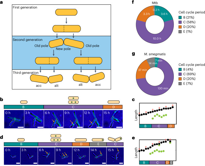
Difficulties in antibiotic treatment of Mycobacterium tuberculosis (Mtb) are partly thought to be due to heterogeneity in growth. Although the ability of bacterial pathogens to regulate growth is crucial to control homeostasis, virulence and drug responses, single-cell growth and cell cycle behaviours of Mtb are poorly characterized. Here we use time-lapse, single-cell imaging of Mtb coupled with mathematical modelling to observe asymmetric growth and heterogeneity in cell size, interdivision time and elongation speed. We find that, contrary to Mycobacterium smegmatis, Mtb initiates cell growth not only from the old pole but also from new poles or both poles. Whereas most organisms grow exponentially at the single-cell level, Mtb has a linear growth mode. Our data show that the growth behaviour of Mtb diverges from that of model bacteria, provide details into how Mtb grows and creates heterogeneity and suggest that growth regulation may also diverge from that in other bacteria.

Fig. 1. Measurement of growth characteristics of Mtb (video set A).

a, Schematic of growth parameters derived from Mtb across generations by time-lapse imaging. Cells loaded into the device (first generation) establish the pole age for the next generations but are excluded from analysis owing to incomplete cell cycle observation. In the second and subsequent generations, all growth features are determined, including Lb, DNA replication initiation (Li), Ld, interdivision time (Td), growth rate (λ), elongation speed $\left(\frac{\mathrm{d}L}{\mathrm{d}t}\right)$ and identification of old and new poles. In the third (and subsequent) generations, we identify accelerators (acc) (n = 173) and alternators (alt) (n = 130). In baseline experiments (video set A), cell cycle timing at the single-cell level is determined using an SSB–GFP reporter strain of Mtb (total cell n = 363). b, Determination of cell cycle state using SSB–GFP. SSB binds to replication forks^,, with green foci indicating ongoing chromosome replication (C period); there were no visible foci before and after replication (B and D periods, respectively). The yellow arrows highlight the foci. Scale bars = 2 µm. c, Single-cell traces of SSB–GFP localization with hourly timepoints corresponding to b. The distance from the x-axis to the black circle represents cell length. The green circles indicate SSB–GFP foci localization along the cell body. The asterisks correspond to the images shown in b. d, Annotation of the cell cycle state in a cell with an E period, in which a small population (11%) initiates replication before division (foci positive). Daughter cells inheriting the foci enter directly into the C period. The yellow arrows highlight the foci, and the white dashed lines outline some individual Mtb cells. Scale bars = 2 µm. e, Single-cell SSB–GFP traces with hourly timepoints corresponding to d. The green circles indicate SSB–GFP foci. The asterisks correspond to the images shown in d. Length in c and e is unitless. f,g, Cell cycle timing in Mtb (f) and M. smegmatis (g). The average time and proportion of each cell cycle period are shown (B: pre-replication, C: DNA replication, D: post-replication, E: new DNA replication after a D period but before division). The M. smegmatis data are from a previous study.

Fig. 2. Growth properties of Mtb and M. smegmatis.

a,b, Distributions of Lb, Ld, Td and elongation speed $\left(\frac{\mathrm{d}L}{\mathrm{d}t}\right)$ are shown for both Mtb (n = 363; video set A) (a) and M. smegmatis (n = 391) (b). The coefficient of variation is shown in the upper right corner of each plot. The centre line of each box-and-whisker plot indicates the median. The left whisker extends from the minimum value to the lower quartile, and the right whisker extends from the upper quartile to the maximum value. The M. smegmatis data are from a previous study. c,d, Growth property distributions are compared between acc and alt cells in Mtb (n of acc = 173, n of alt = 130) (c) and M. smegmatis (n of acc = 193, n of alt = 188) (d). Lb, Ld, elongation speed, growth amount and Td are compared between acc and alt, respectively. Horizontal lines mark the median value for each sample. The M. smegmatis data are from a previous study. P values were calculated using the two-sided, two-tailed Mann–Whitney test. In Mtb, the P values for each comparison are 0.024, 0.66, 0.39, 0.27 and 0.80, respectively (c). The P values for M. smegmatis are 8.29 × 10⁻²³, 6.66 × 10⁻²⁰, 2.20 × 10⁻⁹, 0.0004 and 0.070, respectively (d). Mann–Whitney U = 9,542, 10,908, 10,592, 10,419 and 11,050 in Mtb and 7,576, 8,326, 11,712, 14,335 and 16,207 in M. smegmatis, respectively. e,f, Distributions of division asymmetry in Mtb, M. smegmatis and E. coli. The distributions of division asymmetry in Mtb (e) and M. smegmatis (f) are calculated using the equation Lb of alt cell (daughter cell)/Ld of mother cell. The division symmetry of E. coli is calculated using the equation Lb of daughter cell/Ld of mother cell (e). The M. smegmatis and E. coli data are from previous studies^,. The dashed lines at 0.5 indicate perfect symmetry. The CVs of Mtb, E. coli and M. smegmatis are 12%, 6% and 22%, respectively. *P < 0.05; ***P < 0.001; ****P < 0.0001. NS, not significant.

Fig. 3. Polar growth and growth symmetry in Mtb (measured in video set B).

a, A 5-h-interval image sequence of FDAA-labelled Mtb cells. Individual cells were fully labelled with HADA at the beginning of the time-lapse imaging. The unlabelled area at the poles indicates a newly grown cell wall since the start of the imaging. The white dashed lines outline some individual Mtb cells. Scale bars = 2 µm. b, Schematic diagram of polar growth quantification using FDAA-labelled Mtb. The green area within the cell indicates FDAA (HADA) labelling. The white (unlabelled) area at the poles indicates the new cell wall. The white dashed line indicates septum formation. c, Distribution of growth asymmetry in Mtb. The histogram is fit with a Gaussian. The grey dashed line (score of 0.5) represents symmetric growth (mean value = 0.58, n = 147).

Fig. 4. Linear growth modes.

a, The binned data trend of the growth rate $\left(\frac{1}{L}\frac{\mathrm{d}L}{\mathrm{d}t}\right)$ versus age plot is shown for Mtb data (video set A, n = 363 for unbuffered; video set C, n = 135 for acidic; video set B, n = 248 for neutral condition, using the cells that are born and divided during the video only). The binned data trends decrease with age and are largely consistent with the predicted trends obtained using simulations of linear growth (red lines). b, The binned data trend of the elongation speed versus age plot is shown for Mtb data. The binned data trends are nearly constant, consistent with linear growth simulations (red lines). The dots and error bars indicate mean ± s.e.m. Age in a and b is unitless.

Fig. 5. Growth characteristics at old and new poles.

a–c, Representative examples of different polar growth dynamics (video set B; other examples are shown in Extended Data Fig. 4). The elongation length at each pole is shown as a function of time. The lines represent the best fit to the data and can be either linear or bilinear. a, The new pole starts elongating later than the old pole (NETO). b, Both poles elongate from the beginning of the cell cycle (BEITO). c, The new pole starts elongating before the old pole (OETO). The legend in a also applies to b and c. d, Joint distribution of the timings when the old and new poles start growing in neutral (n = 147) and acidic pH (n = 101) (video set B and C, respectively). e, Distribution of the elongation speed at each pole in neutral and acidic pH (video set B and C, respectively). f, Growth rate and elongation speed versus age in neutral (n = 147) and acidic (n = 101) growth conditions. Simulations of the proposed model are carried out using parameters derived from experimental data. Growth rate trends as a function of age and elongation speed versus age are compared between simulations (black) and experiments (red) for neutral pH and acidic pH conditions. The dots and error bars represent mean ± s.e.m. Note that here we are showing numerical simulations with a comparable number of cells to that used in the experiment, leading to significant fluctuations. These fluctuations can obscure the deviations from linearity predicted by the full model, which accounts for different subpopulations. The model predictions, averaged over a larger population of cells, are shown in Extended Data Fig. 4. Age in f is unitless.

Extended Data Fig. 1. Single-cell traces of SSB-GFP localization (movie set A).

The distance between the x-axis and the black circle indicates cell length. Yellow circles indicate SSB-GFP foci. a-c, Cells with a cell cycle comprised of B-C-D periods. The duration of each period can vary between single cells. d,e, Cells with cell cycle comprised of B-C-D-E periods. Cells with an E period initiate another round of DNA replication before division. The daughter cells of this type of cell lack the B period and enters C directly. f, Example cell with a cell cycle comprising a C and D period. This type of cell cycle occurs in cells whose mother begins replication before division (E period). In cases where foci disappeared for a frame or two due to focus issues and then reappeared, we assumed replication continued until the last foci disappeared. g, Proportional distances between new pole or old pole and SSB foci. The left cartoon illustrates how the proportional distance between SSB and new pole or old pole is calculated. The green circle indicates the location of SSB foci. In each cell, the distance was measured when either one or two SSB foci were present. To calculate the proportional distance, the average distance from either the new or old pole was divided by the length of the cell (for cells with one SSB focus: proportional distance between new pole and SSB = a⁄b; for cells with two SSB foci: proportional distance between new pole and SSB = a⁄c, between old pole and near SSB = b⁄c). On the right, the circles represent the proportional distance between SSB foci and the indicated pole (cell numbers with one SSB focus = 363, cell numbers with two SSB foci = 139). The red horizontal lines mark the median value. Each dot represents a single cell from three biological replicates. P-value was calculated using a two-tailed Mann-Whitney test.

Extended Data Fig. 2. Species-specific growth characteristics in mycobacteria.

a, The average time and proportion of each cell cycle period (B: pre-replication, C: DNA replication, D: post-replication, E: new DNA replication after a D period but before division) are indicated. The BCG and M. smegmatis data are from a previous study. b, Distributions of Lb, Ld, Td, and elongation speed are compared between Mtb (n = 363) and BCG (n = 74). The numbers above the plots and red horizontal lines indicate the median value for each sample. P-values were calculated with the two sided, two-tailed Mann-Whitney test. The p-values for each comparison are 9.36*10⁻³⁹, 8.66*10⁻³⁹, 4.10*10⁻⁰⁶, and 6.56*10⁻²¹, respectively. The BCG data are from a previous study.

Extended Data Fig. 3. Growth characteristics of Mtb during the course of time-lapse imaging (movie set A).

The distributions of Lb and Ld, elongation speed, growth amount, and Td are compared between acc (n = 173) and alt (n = 130), respectively. Dots with green, orange, and gray indicate different biological replicates. Colored dots with black border indicate median values of single dots (single cells) in the same color. Horizontal lines mark the median value of a total population for each sample. P-values were calculated with a two-tailed unpaired t-test.

Extended Data Fig. 4. Single cell growth in NETO, BEITO, and OETO (movie set B).

a and d represent single cells with NETO, b and e represent single cells with BEITO, and c and f represent single cells with OETO. d-f, The snapshots display the length grown at the old pole (green line) and the new pole (red line). The plots next to the snapshots illustrate the best fits for length growth vs. time trajectories. A linear fit best describes the old pole growth of cells (d) and (e), while a bilinear fit is preferred for the cell in (f) based on the $\mathrm{\Delta }\mathit{AIC}$ and $\mathrm{\Delta }\mathit{BIC}$ values. Regarding the new pole growth, a linear fit is preferred for cells (e) and (f), while a bilinear fit is preferred for cell (d).

Extended Data Fig. 5. Growth rate vs. age and elongation speed vs. age plots of each biological replicate (movie set A).

a-c, The binned data trend (blue dots) of growth rate $\left(\frac{1}{L}\frac{\mathit{dL}}{\mathit{dt}}\right)$ vs. age plots are shown for three individual replicates of Mtb data (n = 125, 116, 122, respectively). The binned data trend decreases with age and is largely consistent with the predicted trend obtained using simulations of linear growth (red line). d-f, The binned data trend (blue dots) of elongation speed vs. age plot is shown for the three replicates of Mtb data. The binned data trend is constant consistent with the predicted trend obtained using linear growth simulations. The error bars are presented as mean ± SEM.

References

1. Mitchison, D. A. Role of individual drugs in the chemotherapy of tuberculosis. Int. J. Tuberc. Lung Dis.4, 796–806 (2000). - PubMed
1. Barry, C. E. et al. The spectrum of latent tuberculosis: rethinking the biology and intervention strategies. Nat. Rev. Microbiol.7, 845–855 (2009). - PMC - PubMed
1. Lenaerts, A., Barry, C. E. & Dartois, V. Heterogeneity in tuberculosis pathology, microenvironments and therapeutic responses. Immunol. Rev.264, 288–307 (2015). - PMC - PubMed
1. Cadena, A. M., Fortune, S. M. & Flynn, J. L. Heterogeneity in tuberculosis. Nat. Rev. Immunol.17, 691–702 (2017). - PMC - PubMed
1. Chung, E. S., Johnson, W. C. & Aldridge, B. B. Types and functions of heterogeneity in mycobacteria. Nat. Rev. Microbiol.20, 529–541 (2022). - PMC - PubMed
MeSH terms
LinkOut - more resources