High-Density Recording Reveals Sparse Clusters (But Not Columns) for Shape and Texture Encoding in Macaque V4

Abstract

Macaque area V4 includes neurons that exhibit exquisite selectivity for visual form and surface texture, but their functional organization across laminae is unknown. We used high-density Neuropixels probes in two awake monkeys (one female and one male) to characterize the shape and texture tuning of dozens of neurons simultaneously across layers. We found sporadic clusters of neurons that exhibit similar tuning for shape and texture: ∼20% exhibited similar tuning with their neighbors. Importantly, these clusters were confined to a few layers, seldom "columnar" in structure. This was the case even when neurons were strongly driven and exhibited robust contrast invariance for shape and texture tuning. We conclude that functional organization in area V4 is not columnar for shape and texture stimulus features and in general organization may be at a coarser stimulus category scale (e.g., selectivity for stimuli with vs without 3D cues) and a coarser spatial scale (assessed by optical imaging), rather than at a fine scale in terms of similarity in single-neuron tuning for specific features. We speculate that this may be a direct consequence of the great diversity of inputs integrated by V4 neurons to build variegated tuning manifolds in a high-dimensional space.

Keywords: functional architecture; monkey; neuropixels; object recognition; shape perception; visual cortex.

Figure 1.

Recording methods and visual stimuli. A, A high-density Neuropixels probe (left) was used to study the responses of subpopulations of V4 neurons across cortical laminae. We targeted dorsal V4 on the prelunate gyrus (middle panel). Neurons across laminae (dots in the left panel) had partially overlapping RFs (circles in the right panel) identified during preliminary RF characterization. Visual stimuli were presented at the center of the aggregate RF. FP, fixation point. B, Visual stimuli included 15 two-dimensional shape silhouettes, each presented at eight different rotations in 45° increments. Shapes were presented at two luminance contrast levels (bright or dark) relative to the background. C, Forty naturalistic textures at different orientations (see Materials and Methods) were presented in two versions: original or contrast-reversed (compare last two columns).

Figure 2.

Example recording session: neuronal metrics and CSD. A, Location, waveforms, and interspike interval (ISI) histograms of recorded neurons in penetration M2p6. Left. Location of neurons recorded during this session (n = 24) indicated by the contact closest to the center of mass of waveform amplitudes across contacts. Neuron number (color) is rank-ordered relative to the most superficial neuron. Multiple neurons recorded on the same contact are denoted by larger dots. Right. Spike waveforms from two example neurons (#3, red; #4, blue) recorded on the same set of 14 contacts (left, black squares). Bottom. ISI histograms (N, # of spikes; bin size = 0.2 ms) for four example neurons based on spikes across the entire recording session. Refractory period (2 ms) is indicated by a dashed line. B, Current source density profile along the probe length. Current sink (red) and source (blue) were evaluated by applying current source density (CSD) analysis method to trial-averaged local field (LF) signals evoked by shape stimulus onset (see Materials and Methods). Cross marker indicates the current sink considered to be layer 4 (depth = 1,073 μm, time to current sink = 53 ms after stimulus onset). C, Onset latency of responses to dark stimuli. Latency was quantified as the time to half-peak of the peristimulus time histogram (PSTH) constructed from responses to shape stimuli. For each neuron, spike rasters for all dark stimuli were accumulated and then were smoothed using a Gaussian smoothing window (size of kernel = 4, sigma = 10). Time to half-peak was assessed starting 20 ms after stimulus onset since latencies <20 ms are likely noise. PSTHs were constructed relative to baseline activity, which was quantified as mean activity during the 30 ms time period before stimulus onset. D, Frequency histogram for the average firing rate (baseline-subtracted, x-axis) of each neuron (y-axis) across 120 dark stimuli. Grayscale shows the number of stimuli (log-scale) associated with each firing rate.

Figure 3.

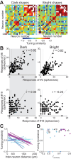
Example recording session: cluster of similarly shape-tuned neurons. A, Tuning similarity in the responses to dark (left) or bright (right) shape stimuli across the set of 24 simultaneously studied neurons in penetration M2p6 (same penetration as in Fig. 2). Similarity values range from −1 (blue) to 1 (red). The white pixels denote neuron pairs for which tuning similarity could not be quantified reliably (due to poor signal-to-noise ratio, see Materials and Methods). Neuron number runs from most superficial (1, purple) to deepest (24, cyan) along the probe. B, Scatter plots relating the responses of two pairs of neurons (top, #3 vs #8; bottom, #18 vs #19; see Fig. 2A) for dark (left) and bright (right) shape stimuli. The top pair shows high tuning similarity (r = 0.82, left; r = 0.82, right), but the bottom does not (r = 0.00, left and r = −0.25, right) even though all four neurons exhibit a broad range of responses that show high tuning invariance (Fig. 3D). The dotted lines indicate baseline FRs. C, Linear regression lines characterize the trend of tuning similarity (y-axis) versus inter-neuron distance (x-axis) for each neuron (line color) and its neighbors (see Materials and Methods). Attenuation of tuning similarity with increasing inter-neuron distance was captured by a positive intercept and a negative slope. The solid and dashed lines indicate regression lines with and without significant intercept. D, Shape tuning invariance (y-axis) versus y-intercept of regression lines in C (x-axis, I_similarity). Filled and open circles indicate neurons with and without significant intercept, respectively.

Figure 4.

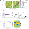
Example session without a cluster of similarly shape-tuned neurons. A, Location of recorded neurons (n = 42) along the probe. Larger dots denote multiple neurons recorded on the same contact. B, Tuning similarity across all pairs of recorded neurons based on the responses to shape stimuli darker (left) or brighter (right) than the background. All other details as in Figure 3A. Evidence of clustered shape tuning is absent. C, Frequency histogram for the average firing rate (baseline-subtracted, x-axis) for each neuron (rows) across the 120 dark shape stimuli. Grayscale shows the number of stimuli (log-scale) associated with each firing rate bin. D, Linear regression lines characterizing the trend of tuning similarity (y-axis) versus inter-neuron distance (x-axis). All other details as in Figure 3C. The y-intercept for the regression line was significantly different from zero for only one neuron (solid line). E, Responses from three example neurons in this session (#7, #18, and #32) for dark (x-axis) versus bright (y-axis) shapes. Baseline-subtracted average firing rates are shown. The solid gray lines indicate identity lines. F, y-intercept of regression lines (x-axis, I_similarity) plotted as a function of shape tuning invariance across contrasts (y-axis). All details as in Figure 3D. Neurons in this penetration did not exhibit shape tuning that was similar to their neighbors (filled), but most neurons did exhibit high shape tuning invariance. Only one neuron with y-axis = 0 showed low reliability in the tuning invariance metric. G, CSD profile constructed from LFP signal evoked with shape stimuli. Cross marker on the current sink (red) considered to be layer 4 was at depth = 570 μm relative to most superficial neuron. Time to current sink = 52 ms after stimulus onset. All other details as in Figure 2B.

Figure 5.

Population results for clustered shape tuning. A, I_similarity (color) for each neuron is illustrated as a function of recorded depth (y-axis) across sessions (columns) sorted according to the probe length over which neurons were recorded. To ensure clarity, green to blue span the 0–0.6 range of I_similarity; values outside of this range were set to either green (for I_similarity< 0) or blue (for I_similarity> 0.6). The asterisks at the top of the panel indicate penetrations with five or more neurons with significant I_similarity. Diamonds indicate 18 penetrations that likely targeted the V4 gyrus (rather than the sulcal bank, see Fig. 8) in M2. Penetrations depicted in Figures 2–4, 6, 7, and 11 are identified. B, Intercept of regression lines (I_similarity) based on tuning similarity for dark (x-axis) versus bright shape stimuli (y-axis). Results from the two sets of stimuli are consistent. C, D, Percentage of neurons with I_similarity significantly different from 0 (C) and mean of I_similarity (D) are plotted on the y-axis as a function of the number of simultaneously studied neurons (x-axis). N denotes the number of penetrations. E, Relationship between the percentage of neurons with I_similarity significantly different from 0 (y-axis) and the recording density (x-axis). Pearson's correlation coefficient, r = 0.236, p = 0.0429. Recording density was evaluated by dividing the distance between the deepest and shallowest neurons by the number of neurons studied within each penetration.

Figure 6.

Tuning similarity based on orientation × SF fits to shape responses. A, I_similarity was constructed from the responses to shape stimuli predicted by a linear weighted sum of 12 Gabor filters. Conventions and color legend are the same as in Figure 5. B, I_similarity based on the orientation × SF fits was positively correlated with I_similarity based on shape responses (Fig. 5A, Spearman's correlation coefficient r = 0.588, p < 0.0001). C, D, Preference for orientation at a coarser scale (top) and I_similarity based on shape responses (bottom) across laminae for two penetrations. Preference for vertical orientation was assessed by the area under the ROC curve, which was constructed from spike count distributions of responses to the spindle-shaped stimulus (Fig. 1, Shape #1) oriented horizontally (0° and 180°) versus vertically (90° and 270°; see Materials and Methods, Feature models). Clustered preference for vertical or horizontal orientations were highlighted with red and blue shading, respectively.

Figure 7.

Tuning for angular position and curvature. A, Tuning for angular position (AP) and curvature (CV) of a subset of recorded neurons (n = 33) that were well fit (goodness of fit r > 0.5) by the 4D angular position × curvature model are shown. Tuning peaks for AP and CV of individual neurons are represented as angular and radial coordinates in this polar plot, respectively. Data points for individual neurons are color-coded by recorded depth (purple, superficial; cyan, deep). B, C, inter-neuron difference of AP (ΔAP; B) and CV (ΔCV; C) is illustrated as a function of inter-neuron distance (μm, x-axis).

Figure 8.

Recording location and its influence on clustered shape selectivity. A, The image of fixed tissue from monkey M2. The image shows indentations created by repeated probe insertions (darker areas in the center). Three solid lines identify anatomical landmarks: STS, superior temporal sulcus; LUS, lunate sulcus; and IOS, interior occipital sulcus. B, Color-coded map shows the RF azimuth from 44 recordings in M2. The black squares identify the eight grid locations where probe penetrations (n = 18) were distant from both horizontal and vertical meridians. C, Percentage of neurons exhibiting significant I_similarity from 18 penetrations (black symbols) through the eight grid locations in B. Results from all other penetrations from both animals are overlaid in gray (same data as in Fig. 5C).

Figure 9.

Population results for clustered texture tuning. A, I_similarity of texture tuning similarity for each neuron (color) is illustrated as a function of recorded depth (y-axis) across 51 penetrations (columns). The blue and green dots identify neurons with and without high texture tuning similarity with neighboring neurons, respectively (see details as in Fig. 5A). The asterisks above the panel indicate penetrations with five or more neurons with significant I_similarity. B, I_similarity from regression lines for tuning similarity based on responses to original textures (x-axis) versus contrast-reversed textures (y-axis). Results from the two sets of stimuli are consistent.

Figure 10.

Effect of recording yield size on the detection of clustered tuning. Number (A) and percentage (B) of neurons with I_similarity significantly different from 0 (y-axis) as a function of the number of simultaneously studied neurons (x-axis). N denotes the number of penetrations. The gray and black circles indicate penetrations where responses to shape and texture were studied.

Figure 11.

Position invariance of tuning similarity. A, Example penetration with a small cluster of similarly tuned neurons (M2p9). Similarity matrices based on the responses to 15 shape stimuli presented at five positions relative to the aggregate RF center are shown. Colored dots at right identify neurons that showed visually evoked responses during preliminary characterization (see B). B, RF center position (x- and y-axes) for the neurons in this recording session plotted as a function of the depth from superficial neuron (z-axis). RF centers were estimated from an automated RF localization procedure (see Materials and Methods). Eight neurons that failed to yield an RF estimate are not depicted. Black circles, aggregate RF. The five stimulus positions (center, north, east, west, and south) are indicated by vertical gray lines. HM, horizontal meridian; VM, vertical meridian. Inset n indicates neuron numbers with quantified RF centers. C, Similarity matrices from a penetration (M2p28) without a cluster of similarly tuned neurons. All other details as in A. D, RF position (x- and y-axes) and depth (z-axis) of neurons recorded for the penetration depicted in C. Details as in B.

Figure 12.

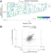
Tuning similarity based on responses at best RF position. A, Single-neuron optimized measure of tuning similarity for the two penetrations depicted in Figure 11A,B (left) and Figure 11C,D (right). For each neuron in each penetration, we first identified the optimal stimulus position as the one associated with the greatest dispersion in responses. We then used the responses from the optimal position to construct a tuning similarity matrix (see Materials and Methods). B, I_similarity computed based on the optimal position (y-axis) versus I_similarity computed in the main shape test (x-axis). Inset N and n indicate penetration and neuron numbers, respectively.

Figure 13.

Simulation: tuning progression and the resulting tuning similarity patterns. A–E, The top row shows shape tuning peaks of model V4 neurons in the angular position × curvature space. Responses of model units to shape stimuli were dictated by a 2D Gaussian function centered at the peak position shown. Curvature runs from −0.5 (moderate concavity) to 1.0 (sharp convexity) and specifies the curvature of the preferred boundary feature. Angular position runs from 0° (pointing right) in a counterclockwise direction and specifies the position of the preferred feature relative to the object center. Different tuning peak progressions (left to right) across 30 model neurons along the length of the probe (purple, superficial; cyan, deep) were considered for each panel. Tuning similarity matrices across model neurons are shown at the bottom. Tuning similarity ranges from −1 (blue, opposite preference) to 1 (red, identical preference). The tuning similarity matrices were constructed by computing the noise-corrected correlation coefficient between modeled spike counts of 30 neurons to 120 shapes used in the main experiment. For each of the 120 shapes, noisy spike counts were modeled for three trial repetitions by implementing Poisson spiking (see Materials and Methods). A, Tuning preference along the curvature dimension (y-axis) gradually shifts from a preference for sharp convexity (curvature = 1) to medium concavity (−0.5) from superficial to deep neurons, while the preferred angular position remained at values around 191° (pointing left). All other parameters of the 2D Gaussian function (SD and amplitude, denoted by circles) were randomly set across neurons. B, Tuning preference along the curvature (y-axis) remains constant at low convexity with small fluctuation along the curvature, while the preferred angular position gradually shifts from a preference for features pointing to the right in a counterclockwise direction. All other details as in A. C, The tuning preference of modeled neurons gradually changes along both the angular position and curvature dimensions. Step sizes of tuning shifts for angular position and curvature were the same as those in A and B. D, Preferred angular position and curvature were chosen at random for individual model neurons. E, Five neurons exhibiting systematic shift of preferred angular curvature from left (180°) in a counterclockwise direction were interleaved among neurons with random peaks.

References

1. Albright TD, Desimone R, Gross CG (1984) Columnar organization of directionally selective cells in visual area MT of the macaque. J Neurophysiol 51:16–31. 10.1152/jn.1984.51.1.16 - DOI - PubMed
1. Bigelow A, Kim T, Namima T, Bair W, Pasupathy A (2023) Dissociation in neuronal encoding of object versus surface motion in the primate brain. Curr Biol 33:711–719.e5. 10.1016/j.cub.2023.01.016 - DOI - PMC - PubMed
1. Bushnell BN, Harding PJ, Kosai Y, Bair W, Pasupathy A (2011) Equiluminance cells in visual cortical area v4. J Neurosci 31:12398–12412. 10.1523/JNEUROSCI.1890-11.2011 - DOI - PMC - PubMed
1. Dagnino B, Gariel-Mathis MA, Roelfsema PR (2015) Microstimulation of area V4 has little effect on spatial attention and on perception of phosphenes evoked in area V1. J Neurophysiol 113:730–739. 10.1152/jn.00645.2014 - DOI - PMC - PubMed
1. David SV, Hayden BY, Gallant JL (2006) Spectral receptive field properties explain shape selectivity in area V4. J Neurophysiol 96:3492–3505. 10.1152/jn.00575.2006 - DOI - PubMed
LinkOut - more resources