A functional microbiome catalogue crowdsourced from North American rivers

Abstract

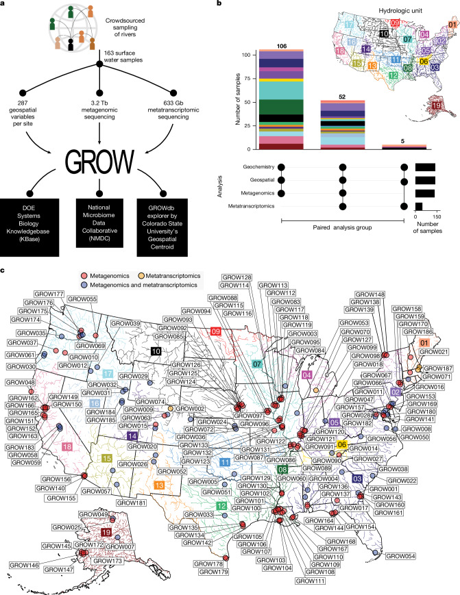
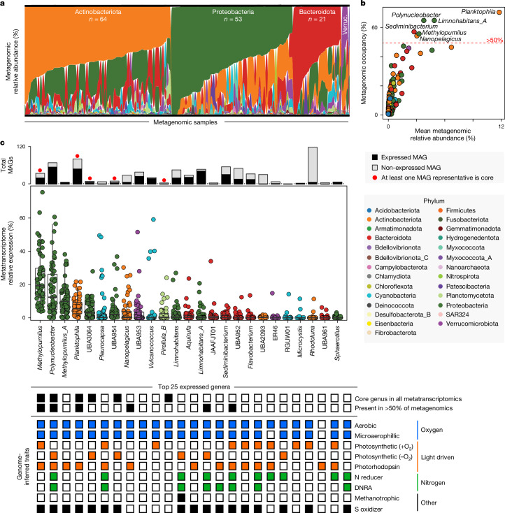
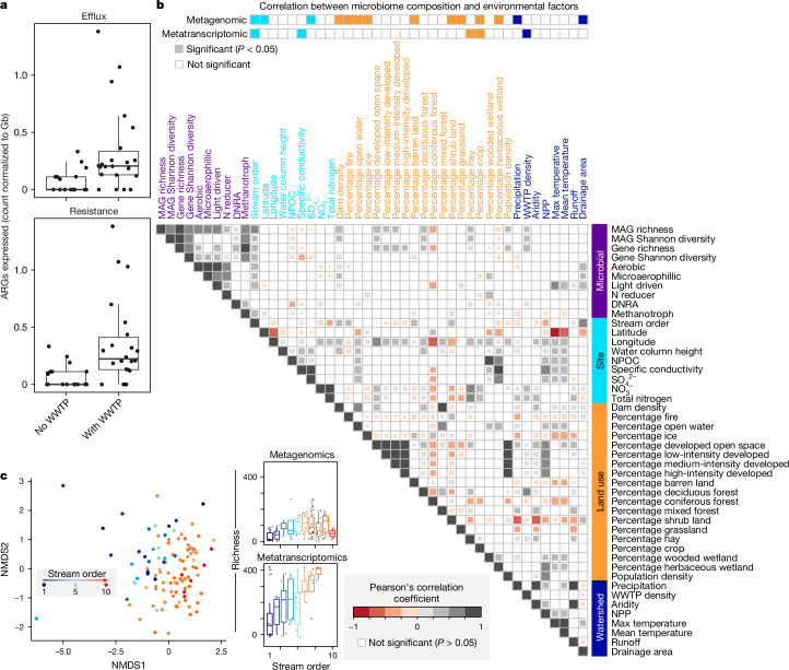
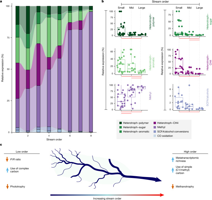
Predicting elemental cycles and maintaining water quality under increasing anthropogenic influence requires knowledge of the spatial drivers of river microbiomes. However, understanding of the core microbial processes governing river biogeochemistry is hindered by a lack of genome-resolved functional insights and sampling across multiple rivers. Here we used a community science effort to accelerate the sampling, sequencing and genome-resolved analyses of river microbiomes to create the Genome Resolved Open Watersheds database (GROWdb). GROWdb profiles the identity, distribution, function and expression of microbial genomes across river surface waters covering 90% of United States watersheds. Specifically, GROWdb encompasses microbial lineages from 27 phyla, including novel members from 10 families and 128 genera, and defines the core river microbiome at the genome level. GROWdb analyses coupled to extensive geospatial information reveals local and regional drivers of microbial community structuring, while also presenting foundational hypotheses about ecosystem function. Building on the previously conceived River Continuum Concept¹, we layer on microbial functional trait expression, which suggests that the structure and function of river microbiomes is predictable. We make GROWdb available through various collaborative cyberinfrastructures^2,3, so that it can be widely accessed across disciplines for watershed predictive modelling and microbiome-based management practices.

Fig. 1. Distributed sampling and sequencing of rivers enabled the construction of the GROWdb.

a, The workflow, denoting the number of samples and the resulting datasets made up of geospatial and microbiome (metagenomics, metatranscriptomics) data. GROWdb data are accessible through KBase, NMDC and the GROWdb Explorer. b, The number of samples with paired data types (denoted as filled black circles below) coloured by hydrologic unit, and the number of samples per analysis. c, GROW sampling across the United States. The points mark the sampling location. Colour coding represents the microbiome analysis performed (metagenomics, red; metatranscriptomics, yellow; paired metagenomics and metatranscriptomics, blue). The boxed numbers and the corresponding river colours indicate hydrologic unit (HUC-2).

Fig. 2. Core lineages and functions across river microbiomes.

a, Phyla metagenomic relative abundance across samples, with each sample organized by the most dominant phyla from top to bottom along the y axis. The samples are grouped by the dominant phyla along the x axis. The Actinobacteriota, Proteobacteria, Bacteroidota and Verrucomicrobiota (Verruc.) phyla are the most dominant across samples. b, The metagenomic relative abundance versus metagenomic occupancy (the percentage of metagenomes that a genus was present in); the points represent each genus in GROWdb and are coloured by phylum. Genera detected in more than 50% of samples (red dashed line) are named. c, The top 25 most transcribed (highest metatranscriptomic expression) genera are shown by box plots, with each point representing a single metatranscriptome (n = 57 metatranscriptomes). The upper and lower box edges extend from the first to third quartile, the centre line represents the median and the whiskers are 1.5× the interquartile range; points outside this range represent outliers. The stacked bar chart above box plots indicates the number of MAGs in GROWdb within each genus and is coloured by detection in metatranscriptomes (black, expressed; grey, non-expressed). A red circle above the bar indicates that one of the genomes was core across metatranscriptomes, as defined as having gene expression in every sample. For each of the top 25 expressed genera, the black boxes represent those that were detected in 100% of metatranscriptomes (core genera) and in more than 50% of metagenomes. The inferred genomic potential of each genus is indicated below, including aerobic respiration (blue), light-driven energy metabolism (orange), nitrogen metabolism (green) and other metabolisms (methanotrophy and sulfur oxidation, black). DNRA, dissimilatory nitrate reduction to ammonium.

Fig. 3. Patterns and drivers of river microbiome composition and function.

a, The number of efflux pumps (top) and ARGs (bottom) expressed at sites without or with impact from WWTPs, normalized to Gb of metatranscriptomic sequencing per sample (n = 43 metatranscriptomes). b, Metagenomic and metatranscriptomic composition, function and diversity were related to 36 selected site, land-use or watershed variables using Mantel tests (top two rows). This was followed with pairwise comparisons using Pearson’s correlation (heat map in b), with only significant values shown, as determined using the two-sided cor.test in R. Variables are coloured by category, including microbial (purple), site or local (light blue), land-use (orange) and watershed metrics (dark blue). For pairwise comparisons of microbial data, metatranscriptomic metrics were used for diversity and function abundance calculations. c, Microbial community diversity was significantly associated with stream order as depicted by non-metric multidimensional scaling of genome resolved metagenomic Bray–Curtis distances (left, beta-diversity) and Pearson correlations of richness to stream order (right, alpha-diversity) with points (n = 105) coloured by stream order. For the box plots, the upper and lower box edges extend from the first to third quartile, the centre line represents the median and the whiskers are 1.5× the interquartile range; points outside this range represent outliers.

Fig. 4. Microbial lifestyle and carbon use are structured along a stream-order gradient.

a, The relative expression of microbial lifestyles (defined in the Methods) across stream-order gradient. b, One-dimensional box plots correspond to data in a, with each point (n = 53) representing a single sample and streams grouped by small (1–3), mid (4–6) and large (7–8) orders. For the box plots, the upper and lower box edges extend from the first to third quartile, the centre line represents the median and the whiskers are 1.5× the interquartile range; points outside this range represent outliers. Significant differences in expression between small-, mid- and large-order streams were determined using Kruskal–Wallis tests and are denoted by horizontal red bars below each plot (P < 0.01). Exact P values are reported in Supplementary Data 4. c, The stream-order model highlights changes in microbial expression from small-order (left) to large-order (right) streams.

Extended Data Fig. 1. Distribution of river characteristics sampled in GROWdb.

A) Heatmap of geospatial and chemical parameters sampled in GROWdb, where columns are environmental and variables and rows are corresponding samples within GROWdb. Each variable has been scaled by subtracting the vector mean for each variable and dividing by its standard deviation. Variables in grey text were determined by FTICR. Blue histogram plots above highlight the distribution of samples for each variable, with high values at the top of the plot. Histogram plots of key variables used throughout the main text including stream order (B) and ecoregion (C) are also shown.

Extended Data Fig. 2. GROWdb comparison to other metagenomics data sources.

A) Sequencing depth comparison of GROWdb metagenomes (n = 158) to SRA metagenomes classified as riverine (n = 222) shows 3x increase in average sequencing depth for GROWdb. Each point represents a single metagenome, with mean and median values listed at the top of the graph. For the boxplot, upper and lower box edges extend from the first to third quartile and the line in the middle represents the median. The whiskers are 1.5 times the interquartile range and every point outside this range represents an outlier. B) Stacked bar chart shows novelty of GROWdb MAGs when compared to GTDB (r207). Each MAG was placed at the highest level of novelty, with no assignment within a taxonomic level (e.g., unnamed family or genus) being highest level of novelty and alpha numeric identifiers being the second highest (e.g., UBA lineages). Bars are coloured by Phylum. C) Stacked bar chart shows the proportion of SRA metagenomes that a GROWdb lineage (95% identity) was detected (black) or not detected (grey) within an SRA environment category. D) The top ten MAGs most frequently detected across river surface water related SRA metagenomes are displayed at the genus level on the bar chart, with colours denoting phyla (key above).

Extended Data Fig. 3. Taxonomic diversity of 2,093 unique surface water metagenome assembled genomes (MAGs) in GROWdb.

A) Cladogram shows GROWdb MAGs taxonomy with each sequential ring noting taxonomy level (Phylum, P; Class, C; Order, O; Family, F). Circle size indicates the number of genomes within a given taxonomy level and is further noted by MAG number inside the circle when sampling at that taxonomic position exceeds 50 MAGs sampled. Colours highlight phylum level taxonomy denoted on the outermost ring. Open triangles represent unnamed lineages within a particular level of taxonomy. B) MAG accumulation curve where the black line represents the mean richness of 100 random permutations and grey shading represents standard deviation. C) One dimensional boxplot displays the environments GROWdb MAGs were detected in across 266,764 metagenomes in the Sequence Read Archive with each point representing a single MAG. Upper and lower box edges extend from the first to third quartile and the line in the middle represents the median. The whiskers are 1.5 times the interquartile range and every point outside this range represents an outlier. Environments are ordered by number of metagenomes GROWdb MAGs were detected in from left to right, with the number of metagenomes also noted along the x-axis. Freshwater related environments are highlighted in blue.

Extended Data Fig. 4. GROWdb comparison to global freshwater MAGs.

In order to compare GROWdb MAGs in this study derived from United States watersheds, we have compiled MAGs from other biogeography studies with freshwater MAGs^–, as well as included 1,286 additional MAGs derived from 23 metagenomes released in this study, including 6 countries beyond the United States (UK, Canada, Italy, Germany, Israel, Republic of the Congo). A) Area plot shows the dereplication results of 9,798 MAGs from freshwater sources (lakes and rivers) at 99% identity. This dereplication status, with winner defined as the best MAG representative of the cluster, is reported by outline colour with black outline denoting winner and grey outline denoting loser. The area plot within these sections has area size proportional to MAGs recovered, divided first by study (colour in legend), then by country (noted on area plot). B) Stacked bar chart summarizes area plot in A by study, with GROW contributing the most representative MAGs (dRep winners). C) Venn diagram shows the number of MAG representatives (dRep winners) derived from rivers only (does not include lakes) by location, with USA being compared to Non-US sites. Circle area is sized by number of MAGs. D) Nayfach, et al. is a comprehensive catalogue of Earth’s microbiomes that includes 52,215 MAGs, of which we retain 5,336 MAGs from aquatic freshwater environments for our global comparison, excluding soil, sediment, and wastewater related habitats within the aquatic freshwater ecosystem to more directly compare to surface water GROWdb. Pie chart shows the breakdown of sample types for this subset of MAGs, highlighting that a majority are derived from lake systems. E) Bar chart shows clustering of MAGs from other studies with GROWdb non-US studies, with bars coloured by study. F) Venn diagram compares the number of MAG representatives (dRep winners) derived from rivers and lakes across studies, with circle area sized by number of MAGs. Stacked bar chart below summarizes these results by study. All data for this comparison is reported in Supplementary Data 2 (tab 5), with MAG files available at Zenodo.

Extended Data Fig. 5. Metabolic trait assignment ruleset.

Each trait is defined by a set of genes and the percent of genes required for that function. Lines flow from the genome (top black box) to traits (ovals), passing through boxes of gene requirements to be consider TRUE for that particular trait.

Extended Data Fig. 6. Gene level expression across rivers.

Genes detected in more than 50% of metatranscriptomes, with gene functions (n = 365) grouped by broad categories (n = 9, A) and refined to subcategories (n = 41, B). Thickness of lines and line order in A show the number of functions within a particular category (right) and subcategory (left). A and B are linked by subcategory number (1–41). For each of the 41 subcategories, the number of genes and occupancy defined as the percentage of samples detected across metatranscriptomes is shown by bar charts. Hypothetical and genes with unknown annotations are not shown, albeit 21 genes with these annotations were considered core or expressed in all metatranscriptomes. C) Focusing on carbon, carbohydrate-active enzyme (CAZyme) family gene expression is shown across river metatranscriptomes (n = 57) as log-transformed expression (geTMM). In the box plot, upper and lower box edges extend from the first to third quartile and the line in the middle represents the median. The whiskers are 1.5 times the interquartile range and every point outside this range represents an outlier. D) The prevalence of each CAZyme family across the metatranscriptomes is shown by stacked bar plots, which represent the fraction of river metatranscriptomes with expression for each family, with bar colour corresponding to river size as denoted in the legend. The dotted line marks 50% of metatranscriptome samples. At right, the substrate type for each CAZyme family is given based on the DRAM metabolism summary; see Shaffer and Borton et al for substrate logic. If more than one box is present, the CAZyme family can act upon multiple substrate types.

Extended Data Fig. 7. GROWdb membership and structure across geospatial parameters.

A) Stacked bar chart of the singleM profiles of GROWdb metagenomic reads, with bars coloured by domain. By domain, the most reads are assigned to the Bacteria (mean=91.1%), followed by Eukaryota (mean=6.1%), Archaea (mean=2.6%), and Unknown (mean=0.2%). B) Correlations of Patescibacteria relative abundance (metagenomics, top) and expression (metatranscriptomics, bottom) with stream order. Correlation significance was tested in R using cor.test (two-sided), with p-values shown. C) Permutational analysis of variance (PERMANOVA) results for metagenomes (metaG) and metatranscriptomes (metaT) indicate that drivers of community structure and expression, respectively. These drivers and their interactions explain 68% of the metagenome and 41% of the metatranscriptome variance. Bar height represents the R², with green bars denoting significant drivers (p < 0.05), while black bars are not significant drivers. D) Sparse Partial Least Squares (sPLS) regressions show significant function (top) and MAG level (bottom) expression predictions of watershed maximum temperature, with key variables (Variable Importance Projection >1) denoted in bar graphs below. Fitted regression line is shown with grey shading representing 95% confidence interval. E) Non-metric multidimensional scaling of genome resolved metagenomic Bray-Curtis distances shows clustering of microbial communities by ecoregion (classified by Omernik II), with sampling location depicted on map above (mrpp, p < 0.001). Abbreviations: NPOC, Non-Purgable Organic Carbon; DNRA, Dissimilatory Nitrite Reduction to Ammonia; WWTP Density, Waste Water Treatment Plant Density; NPP, Net Primary Production. F) Non-metric multidimensional scaling of genome resolved metagenomic Bray-Curtis distances shows clustering of microbial communities by hydrological unit (HUC-2), with sampling location depicted on map on Fig. 1c.

Extended Data Fig. 8. GROWdb inventory of Emerging Contaminant Genes.

A) Heatmap shows the genomic potential for emerging contaminant transformation categories by genus, with number of genes normalized to the number of genomes within a genus and scaled by column. Black boxes indicate no detection of a related gene, while red box outlines indicate expression of a gene within at least six metatranscriptomes. B) Several genera encoded the potential for Terephthalate and Phthalate microplastic related metabolisms, with the entire pathway from polyethylene terephthalate (PET) and Phthalate shown. Heatmap corresponds to the pathway with steps 1–7, where box colour indicates the number of genes encoded per genus. Red outlines indicate expression of a gene within at least six metatranscriptomes. C) Emerging contaminant gene expression categories were related to land use, with significant relationships detected among the percent of the watershed classified as low-intensity, urban impacted shown by horizontal red bars (p-value < 0.05). Each point represents a single metatranscriptome (n = 43). Boxplot upper and lower box edges extend from the first to third quartile and the line in the middle represents the median. The whiskers are 1.5 times the interquartile range and every point outside this range represents an outlier. A similar trend was shown with high-impact urban land use, but lacked power based on number of samples. Significance (p-value < 0.05) is noted by red bar.

Extended Data Fig. 9. GROWdb metagenomic analysis pipeline and results.

A) Metagenomic pipeline for GROWdb that resulted in three assemblies per sample (A, B, and F), with all parameters and version used outlined in methods and on GitHub (10.5281/zenodo.11041178). B) Stacked bar graph shows the number of medium (MQ) and high (HQ) quality dereplicated MAG representatives recovered from each assembly type. C) Bar graph shows the number of singleton dereplicated MAG representatives from each assembly type. D) Venn diagram compares the number of dereplicated MAG cluster representatives (dRep winners) recovered from each assembly type with overlaps indicating MAGs within the same cluster were recovered from multiple assembly types.

References

1. Vannote, R. L., Minshall, G. W., Cummins, K. W., Sedell, J. R. & Cushing, C. E. The river continuum concept. Can. J. Fish. Aquat. Sci.37, 130–137 (1980).
1. Wood-Charlson, E. M. et al. The National Microbiome Data Collaborative: enabling microbiome science. Nat. Rev. Microbiol.18, 313–314 (2020). - PubMed
1. Arkin, A. P. et al. KBase: the United States Department of Energy Systems Biology Knowledgebase. Nat. Biotechnol.36, 566–569 (2018). - PMC - PubMed
1. Cavicchioli, R. et al. Scientists’ warning to humanity: microorganisms and climate change. Nat. Rev. Microbiol.17, 569–586 (2019). - PMC - PubMed
1. Hutchins, D. A. & Fu, F. Microorganisms and ocean global change. Nat. Microbiol.2, 17058 (2017). - PubMed