Learning high-accuracy error decoding for quantum processors

Abstract

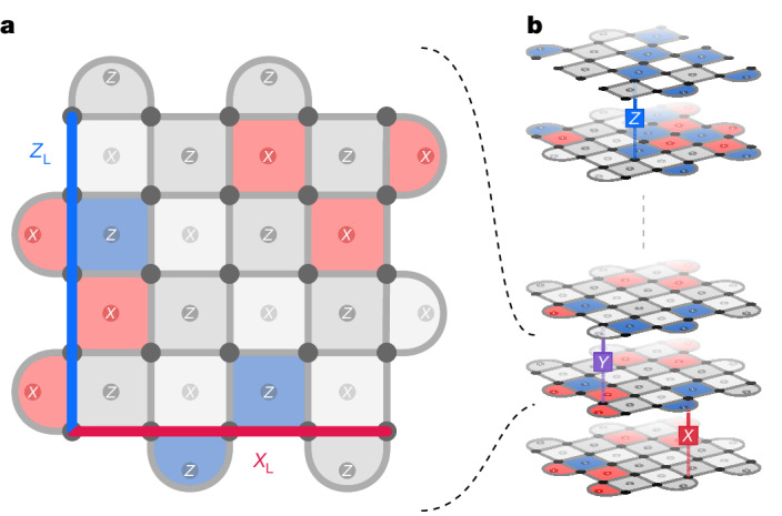
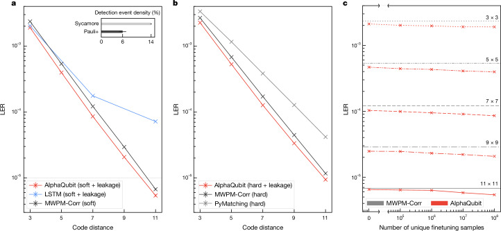
Building a large-scale quantum computer requires effective strategies to correct errors that inevitably arise in physical quantum systems¹. Quantum error-correction codes² present a way to reach this goal by encoding logical information redundantly into many physical qubits. A key challenge in implementing such codes is accurately decoding noisy syndrome information extracted from redundancy checks to obtain the correct encoded logical information. Here we develop a recurrent, transformer-based neural network that learns to decode the surface code, the leading quantum error-correction code³. Our decoder outperforms other state-of-the-art decoders on real-world data from Google's Sycamore quantum processor for distance-3 and distance-5 surface codes⁴. On distances up to 11, the decoder maintains its advantage on simulated data with realistic noise including cross-talk and leakage, utilizing soft readouts and leakage information. After training on approximate synthetic data, the decoder adapts to the more complex, but unknown, underlying error distribution by training on a limited budget of experimental samples. Our work illustrates the ability of machine learning to go beyond human-designed algorithms by learning from data directly, highlighting machine learning as a strong contender for decoding in quantum computers.

Fig. 1. The rotated surface code and a memory experiment.

a, Data qubits (grey circles) on a d × d square lattice (here shown for code distance d = 5) are interspersed with X and Z stabilizer qubits (X and Z in circles). The logical observables X_L (Z_L) are defined as products of X (Z) operators along a row (column) of data qubits. b, In a memory experiment, a logical qubit is initialized, repeated stabilizer measurements are performed and then the logical qubit state is measured. During the experiment all qubits and operations are subject to errors (here symbolically shown as bit (X), phase (Z), and combined bit and phase flips (Y) acting on individual data qubits from time step to time step).

Fig. 2. Error correction and training of AlphaQubit.

a, One error-correction round in the surface code. The X and Z stabilizer information updates the decoder’s internal state, encoded by a vector for each stabilizer. The internal state is then modified by multiple layers of a syndrome transformer neural network containing attention and convolutions. The state at the end of an experiment is used to predict whether an error has occurred. b, Decoder training stages. Pretraining samples come either from a data-agnostic SI1000 noise model, or from an error model derived from experimental data using p_ij or XEB methods^,.

Fig. 3. Logical error per round on the 3 × 3 and 5 × 5 Sycamore experiment.

All AlphaQubit results (both pretrained and finetuned) are for ensembles of 20 models. All results are averaged across bases, even and odd cross-validation splits, and, for the 3 × 3 experiments, the location (north, east, south, west (NESW)), and are fitted across experiments of different durations. a, The 1 − 2 × logical error versus error-correction round for code distance-3 and distance-5 memory experiments in the Sycamore experimental dataset for the baseline tensor-network decoder (black), our decoder (red) and three variants of MWPM (shades of grey). The LER is calculated from the slope of the fitted lines. The error bars are the 95% confidence interval. b, LERs of our decoders and other published results for the Sycamore experiment data. We also show the performance of an LSTM model pretrained on XEB DEM data. Error bars are standard bootstrap errors. c, LERs of our decoder pretrained on different noise models, and after finetuning on experimental data. Error bars are standard bootstrap errors.

Fig. 4. Larger code distances and finetuning accuracy trade-off.

a,b, LER of different decoders for Pauli+ noise at different code distances. For each code distance, our decoder (red) is finetuned on 100 million samples from this noise model after pretraining on a device-agnostic circuit depolarizing noise model (SI1000). MWPM-Corr (black) and PyMatching (grey) are calibrated with a DEM tuned specifically to the Pauli+ noise model with soft information. The error bars are bootstrap standard errors. a, Soft decoder inputs. Inset: detection event density of the Pauli+ simulation compared with the Sycamore experimental samples (error bars are standard error of the mean). b, Hard decoder inputs. c, LER of AlphaQubit (soft inputs) pretrained on SI1000 noise and finetuned with different number of unique Pauli+ samples at code distances 3–11.

Fig. 5. Generalization to larger number of error-correction rounds at code distance 11.

a,b, The 1 − 2 × logical error after up to 100,000 error-correction rounds (a) and the corresponding LER (b) for PyMatching (grey), MWPM-Corr (black) and AlphaQubit (red) pretrained on SI1000 samples up to 25 rounds and finetuned on 10⁸ distance-11 Pauli+ simulated experiments of 25 rounds. Both finetuning and test samples are Pauli+. We plot LER values only where the corresponding 1 − 2 × logical error value is above 0.1. The error bars are bootstrap standard errors.

Fig. 6. Using the network’s output as a confidence measure for post-selection.

Calibration and post-selection data are evaluated on 10⁹ Pauli+ simulated experiments. a, Example calibration plot at distance 5 (green continuous line) and distance 11 (purple continuous line), with small but present error bars for s.e.m. The black dashed line represents a perfectly calibrated classifier. b, LER versus the fraction of low-confidence experiments discarded. Error bars are s.e.m. from values in each bin (visible for a LER ≲ 10⁻⁸).

Extended Data Fig. 1. Stabilizer readout circuit for a 3 × 3 XZZX rotated surface code in the Z basis.

(a) Common X and Z stabilizer readout for the XZZX code. Here, the four first lines (a-d) are the data qubits surrounding a stabilizer qubit (last line), which has been reset to $\mid 0⟩$. (b) Relative strength of noise operations in an SI1000 circuit depolarizing noise model, parameterized by p. (c) Corresponding circuit depolarizing noise gate and error schema. Black dots indicate data qubits, gray dots indicate X/Z stabilizer qubits, as detailed in Fig. 1a. $\mathfrak{D}$ (yellow blocks) labels single- or two-qubit depolarizing noise, and $\mathfrak{X}$ labels a bit flip channel. M, R, and MR are measurements, reset, and combined measurement and reset in the Z basis. H is a Hadamard gate, and CZ gates are indicated by their circuit symbol.

Extended Data Fig. 2. Noise and event densities for datasets used.

(a) Simplified I/Q noise with signal-to-noise ratio SNR = 10 and normalised measurement time t = 0.01. Top plot: point spread functions when projected from its in-phase, quadrature, and time components onto a one-dimensional z axis. Shown are the sampled point spread functions for $\mid 0⟩$ (blue), $\mid 1⟩$ (green), and a leaked higher-excited state $\mid 2⟩$ (violet). Bottom plot: posterior sampling probability for the three measurement states, for prior weights w₂ = 0.5%, w₀ = w₁ = 49.75%. (b) Event densities for different datasets and the corresponding SI1000 p-value. We indicate the event density of the different datasets in the top x-axis, with a non-linear scale. The detector error models are fitted to the Sycamore surface code experiment. All datasets use the XZZX circuit variant of the surface code (with CZ gates for the stabilizer readout, ‘The rotated surface code’ in Methods, Extended data Fig. 1). As we are never compiling between gatesets, there is no implied noise overhead; these are the final event densities observed when sampling from the respective datasets. For datasets with soft I/Q noise, the plots above show the average soft event density as explained in ‘Measurement noise’ in Methods.

Extended Data Fig. 3. Individual fits of logical error per round for 3 × 3 and 5 × 5 memory experiments.

For the p_ij-DEM pretrained model.

Extended Data Fig. 4. The neural network architecture designed for surface code decoding.

(a) 5 × 5 rotated surface code layout, with data qubits (dark grey dots), X and Z stabilizer qubits (labelled light grey dots, or highlighted in blue/red when they detect a parity violation) interspersed in a checkerboard pattern. Logical observables Z_L and X_L are shown as bold lines on the left and bottom grid edges respectively. (b) The recurrent network iterates over time updating a representation of the decoder state and incorporating the new stabilizers at each round. Three parallel lines indicate a representation per stabilizer. (c) Creation of an embedding vector S_ni for each new stabilizer i = 1, …, d² − 1 for a distance d surface code. (d) Each block of the recurrent network combines the decoder state and the stabilizers S_n = (S_n1, …, S_nM) for one round (scaled down by a factor of 0.7). The decoder state is updated through three Syndrome Transformer layers. (e) Each Syndrome Transformer layer updates the stabilizer representations through multi-headed attention optionally modulated by an (optional) learned attention bias followed by a dense block and dilated 2D convolutions. (f) Logical errors are predicted from the final decoder state. The triple lines marked with * indicate a representation per data qubit.

Extended Data Fig. 5. Further architecture details.

(a) Attention bias visualisation. Attention bias logits of the four heads of the first Syndrome Transformer layer of our decoder model pretrained on 5 × 5 DEM in the Z basis. We obtain the logits by combining the learned attention bias embedding with all-zero stabilizer values. The 24 × 24 attention logit matrices are each visualized as one grid per stabilizer, laid out according to the physical layout of the attending stabilizer qubits. Each grid shows the logits for the attention to each stabilizer, with self-attention highlighted with a black square. (b) Architecture of the network when predicting labels at every round. S_n are the stabilizer representations as explained in Extended data Fig. 4b, where the primed quantities $S{\prime }_n$ indicate the embeddings are computed using different embedding parameters and based only on the stabilizers in the experiment basis computed from the final data qubit measurements (‘Input representation’ in Methods).

Extended Data Fig. 6. Calibration of AlphaQubit’s outputs and generalization to longer experiments for code-distances 3–11.

(a) Calibration for Pauli+ generated data with SNR = 10, t = 0.01, and 0.1% stabilizer qubit leakage chance. (b) Calibration histogram of predicted probabilities. The predictions are grouped into correct (blue) and incorrect (red) before building the histogram, and then binned into “certainty” bins depending on their distance from a 50: 50 prediction, i.e. by ∣1/2 − p∣ for a predicted probability p. For all code distances, wrong predictions have a lower certainty. Correct predictions concentrate around the interval edges, i.e. at probabilities 0 and 1, resulting in a high certainty. (c) Generalization to longer experiments. 1 - 2 × logical error and logical error rates for networks pretrained and finetuned on datasets for up to 25 error detection rounds but applied to decoding experiments of longer durations. We only plot logical error rates where the corresponding 1 - 2 × logical error are greater than 0.1. The data is generated from the same simulated experiments, stopped at different number of rounds.

Extended Data Fig. 7. Further result details on Sycamore and scaling experiments, and decoder speed.

(a) Decoding time per error correction round vs. code distance. The hatched region for d > 11 indicates that while AlphaQubit is the same for all code-distances, it has not been trained or shown to work beyond d = 11. The line is a least squares fit to a × d^exponent, and the shaded region marks a 95% CI. Timing of uncorrelated matching (PyMatching). Times for PyMatching use a current CPU (Intel Xeon Platinum 8173M) and for AlphaQubit use current TPU hardware with batch size 1. (b) LER of a decoder trained jointly on distances 3–11, as compared to decoders trained solely on the individual code distances (both pretrained only, see ‘Decoding at higher distances’ and ‘Pauli+’ in Methods). Uncertainty is bootstrap standard error (9 resamples). The model and training hyperparameters are identical in both cases, but for the joint code distance-trained decoder we swap the index embedding for a relative positional embedding, where each stabilizer position (normalized to [−1, 1] × [−1, 1]) is embedded (‘Input representation’ in Methods). (c) Number of pretraining samples until the individual models (pre ensembling) achieve the given LER (relative to the lowest-achieved LER, the latter shown as brown line). The dashed line indicates when the training was stopped (see ‘Termination’ in Methods). Error bars are 95% CI (N = 15). (d) Performance improvement by ensembling multiple models, where we show the p_ij-pretrained model for the Sycamore experiments (XEB and SI1000 variants show about the same improvement). (e) Average error suppression factors Λ for Pauli+ experiment. The error suppression factor is computed from the data in Fig. 4, via the geometric average ${\overline{\mathrm{\Lambda }}}_{3/11}={\left({\mathit{ϵ}}_3/{\mathit{ϵ}}_{11}\right)}^{1/4}$, for a logical error per round ϵ₃ at code distance 3, and ϵ₁₁ at distance 11, respectively.

Extended Data Fig. 8. Network and training hyperparameters.

(a) Noise curriculum parameters used in pretraining for the Sycamore experiment. (b) Hyperparameters of the network architecture. (c) The dilations of the three 3 × 3 convolutions in each syndrome transformer layer and the experiment learning rates are determined by the code-distance of the experiment. (d) Hyperparameters for finetuning of the scaling experiment. The learning rate for finetuning was the initial learning rate for the code-distance from Extended data Fig. 8c scaled by the factor dependent on the training set size. The finetuning cosine learning rate schedule length was code distance × 2/3 × 10⁸ samples.

Extended Data Fig. 9. Ablations: The effect of removing or simplifying decoder architecture elements.

Decoder performance under ablations (white bars) compared to the baseline, ordered by mean LER. The blue bars indicate the model used for the experiments. (a) For 5 × 5p_ij DEM training, averaged across bases (X and Z) and the two cross-validation folds. The red horizontal line represents the performance of the finetuned ensemble. Error bars represent bootstrap standard errors from individual fidelities (499 resamples). (b) For 11 × 11 Pauli+ training. Error bars represent estimated mean error (N = 5). (c) Effect of ablations in performance and data efficiency. Decoding performance of the best performing subset of ablations for 5 × 5 DEM and 11 × 11 Pauli+. Colors indicate the number of training samples required for reaching performance parity with PyMatching for 11 × 11 Pauli+.

References

1. Shor, P. W. Scheme for reducing decoherence in quantum computer memory. Phys. Rev. A52, R2493–R2496 (1995). - PubMed
1. Gottesman, D. E. Stabilizer Codes and Quantum Error Correction. PhD thesis, California Institute of Technology (1997).
1. Fowler, A. G., Mariantoni, M., Martinis, J. M. & Cleland, A. N. Surface codes: towards practical large-scale quantum computation. Phys. Rev. A86, 032324 (2012).
1. Google Quantum AI. Suppressing quantum errors by scaling a surface code logical qubit. Nature614, 676–681 (2023). - PMC - PubMed
1. Feynman, R. P. Simulating physics with computers. Int. J. Theor. Phys.21, 467–488 (1982).
LinkOut - more resources