A Mathematical Model for Wind Velocity Field Reconstruction and Visualization Taking into Account the Topography Influence

Abstract

In this paper, we propose a global modelling for vector field approximation from a given finite set of vectors (corresponding to the wind velocity field or marine currents). In the modelling, we propose using the minimization on a Hilbert space of an energy functional that includes a fidelity criterion to the data and a smoothing term. We discretize the continuous problem using a finite elements method. We then propose taking into account the topographic effects on the wind velocity field, and visualization using a free library is also proposed, which constitutes an added value compared to other vector field approximation models.

Keywords: current/wind velocity field approximation; vector flow visualization; wind velocity field modelling.

Figure A1

BFS rectangle finite element.

Figure A2

Affine transformation to compute the basis function of any point using the basis function of the reference finite element.

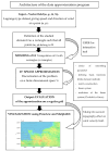
Figure 1

Global view of the approximation framework.

Figure 2

Horizontally, we consider that air streams begin to rise upstream of an obstacle at a distance such that d = h × cot(a/2), with h being the height of the obstacle and a the angle of the slope.

Figure 3

Top: considered parameters for hills and ridges (source: [13]). Bottom: corresponding values of parameter s.

Figure 4

Usual examples of compass wind and wind rose.

Figure 5

Example of an obstacle given by the function f in (10); the arrow gives the considered wind direction (eastern wind). We also give the colormap of the topographic coefficients associated with the east wind direction.

Figure 6

Color map of topographic coefficients associated with a northeast wind direction. The arrow gives the considered wind direction.

Figure 7

Color map of topographic coefficients associated with a west wind direction. The arrow gives the considered wind direction.

Figure 8

Color map of topographic coefficients associated with a southeast wind direction. The arrow gives the considered wind direction.

Figure 9

Top: case of cliffs or escarpments [13]. Bottom: equivalent method to compute orographic coefficients (as we did for hills and ridges).

Figure 10

Studied zone (northwest France). Anemometers located in Caen, Octeville, Rouen, Beauvais, Abbeville and Le Touquet were selected.

Figure 11

Example of a wind dataset for a given time step. The location is northwest France; the data are from anemometers located at six different airports.

Figure 12

We give two different approximations using the model given in Section 2 of the wind velocity field using a 4 × 4 finite element grid (a) and a 3 × 3 finite element grid (b). Colors indicate wind speed (same colormap as on Figure 11).

Figure 13

Topographic map of the studied zone (Normandy Region, France) (a). Wind vector field (approximated from the six different Meteo France locations at airports) on the topographic map (b).

Figure 14

Visualization of a vector flow in Normandy, including the topography effect using Matplotlib (http://lmi.insa-rouen.fr/images/contenu/Movies/Test.gif accessed on 1 November 2024).

Figure 15

Example of visualization of marine currents in Rouen, France. Arrows indicate directions and speed (following length of the arrow) of the current. Visualization is performed using Matplotlib. (http://lmi.insa-rouen.fr/images/contenu/Movies/Rouen.gif accessed on 1 November 2024).

Figure 16

Example of the location of data in a Lidar dataset.

Figure 17

Different streamlines to visualize a vector flow can be used (Short streamlines on the left and long streamlines in the middle. On the right, this is an image we can obtain using the “streamline algorithm” of [15]).

References

1. Gout C., Lambert Z., Apprato D. Data Approximation: Mathematical Modelling and Numerical Simulations. EDP Sciences; Les Ulis, France: 2019. 168p.
1. Dzhabrailov A.S., Klochkov Y.V., Marchenko S.S., Nikolaev A.P. The finite element approximation of vector field in curvilinear coordinates. Russ. Aeronaut. 2007;50:115–120. doi: 10.3103/S1068799807020018. - DOI
1. Benbourhim M.N., Bouhamidi A. Approximation of vector fields by thin plate splines with tension. J. Approx. Theory. 2005;136:198–229. doi: 10.1016/j.jat.2005.07.005. - DOI
1. Benbourhim M.N., Bouhamidi A. Pseudo-polyharmonic vectorial approximation for div-curl and elastic semi-norms. Numer. Math. 2008;109:333–364. doi: 10.1007/s00211-008-0146-x. - DOI
1. Dodu F., Rabut C. Vectorial interpolation using radial-basis-like functions. Comput. Math. Appl. 2002;43:393–411. doi: 10.1016/S0898-1221(01)00294-2. - DOI
LinkOut - more resources