Comprehensive characterization of gas dynamic virtual nozzles for x-ray free-electron laser experiments

Abstract

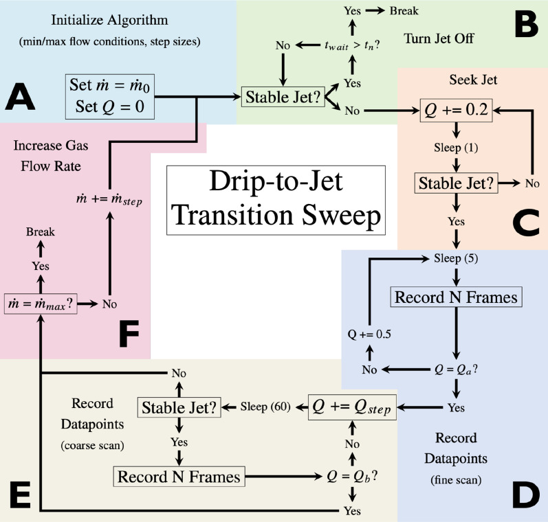
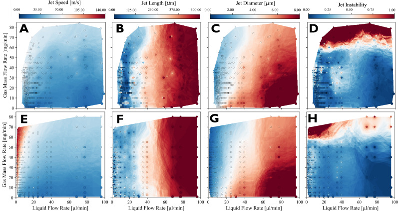
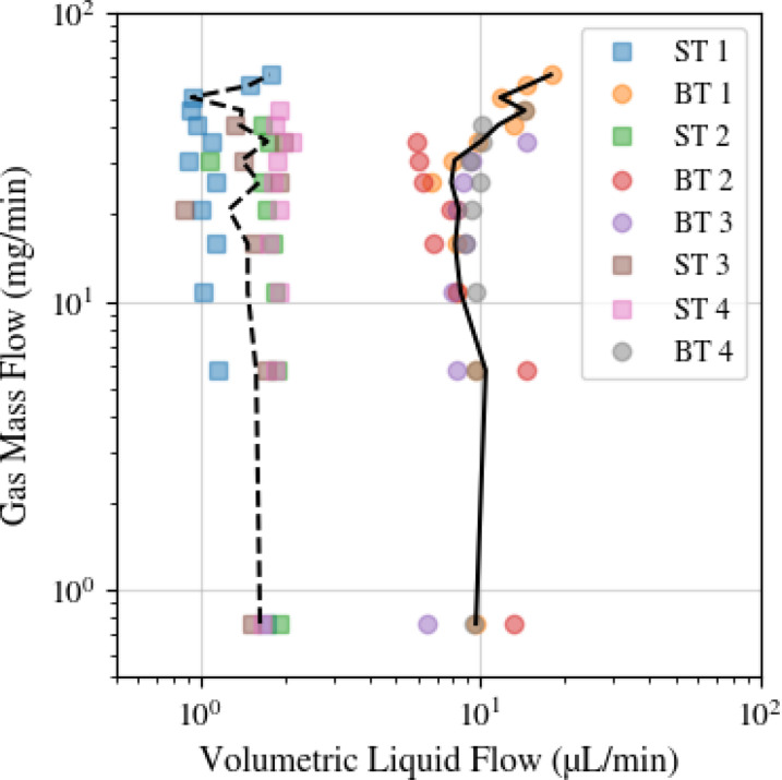
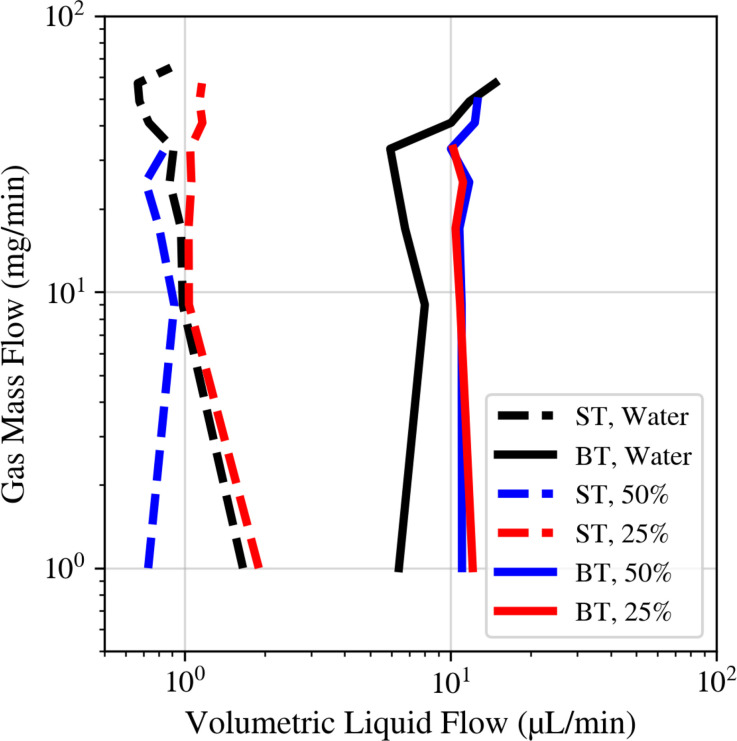
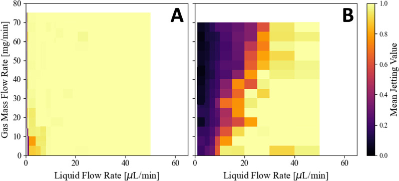
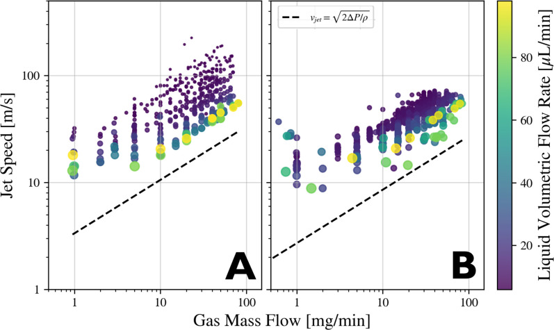
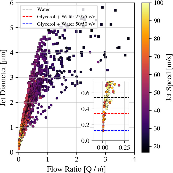
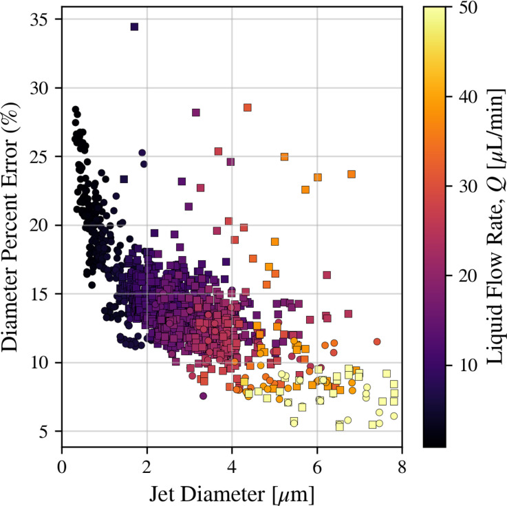
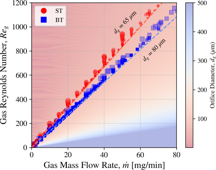
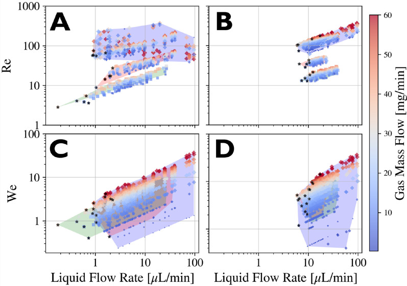
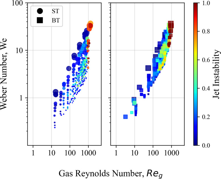
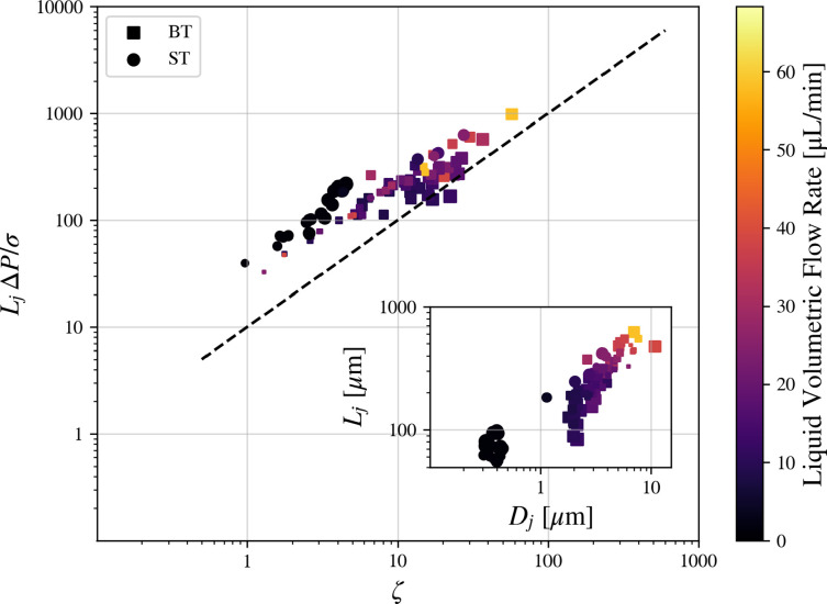
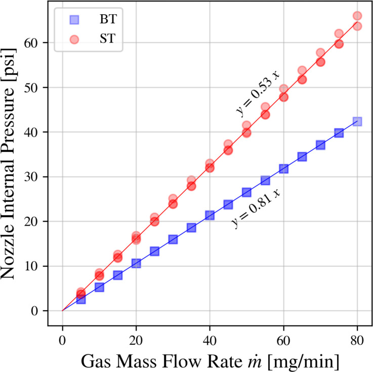
We introduce a hardware-software system for rapidly characterizing liquid microjets for x-ray diffraction experiments. An open-source python-based software package allows for programmatic and automated data collection and analysis. We show how jet speed, length, and diameter are influenced by nozzle geometry, gas flow rate, liquid viscosity, and liquid flow rate. We introduce "jet instability" and "jet probability" metrics to help quantify the suitability of a given nozzle for x-ray diffraction experiments. Among our observations were pronounced improvements in jet stability and reliability when using asymmetric needle-tipped nozzles, which allowed for the production of microjects smaller than 250 nm in diameter, traveling faster than 120 m/s.

FIG. 1.

A two-pulse triggering scheme, a technique known as “frame straddling.”

FIG. 2.

Nozzle testing station flow diagram. Hardware Interfaces and Odysseus software are open-source.

FIG. 3.

Needle tip (ST) and blunt tip (BT) nozzle sectional views, with gas (yellow) and liquid (blue) lines labeled. (a) 65  $\mu$m gas orifice diameter, (b) 50  $\mu$m in diameter liquid channel coming to a point in a hypodermic-syringe-type fashion, (c) 80  $\mu$m gas orifice diameter, and (d) 100  $\mu$m in diameter liquid channel.

FIG. 4.

Definitions of key jet characteristics. Here, $l_j$ is the jet length, $D_j$ is the jet diameter, $\theta$ is the angle from a “straight” jet, and $\varphi$ is the droplet dispersion angle. $x_{IP}$ is the “interaction point,” measured a distance dx from the nozzle tip. The IP is required for the jet instability measure.

FIG. 5.

Standard image processing steps with an example dataset. (b)–(d) show the image cleanup steps, while (e) visualizes the segmentation step. In (e), methods are available to automate the nozzle tip ( $x_0$, red dashed line) and transition region ( $x_1$, green dashed line) index positions. As a simple example of one of the methods, a projected image is displayed in (e) (black solid line), where the individual droplets, continuous jet, and nozzle tip can be easily seen. The blue solid line indicates the jet fit, determined using a Hough transform method for line fitting.

FIG. 6.

A birds-eye-view showing an overlay of many jet images from a dataset with varying gas flow rate. The image stack is sorted by increasing gas flow rate, then translated horizontally by a set distance to give the time-series-style view. When the gas mass flow rate reaches approximately 70 mg/min, the onset of whipping is observed. Jets in this visual were produced with a liquid volumetric flow rate of approximately 5  $\mu$l/min. The index positions for the nozzle tip and breakup region were automatically determined using methods from the microjet_analysis repository. Breaks in the jet, particularly seen near the nozzle tip in the range 45–90 mg/min, and the missing droplets in the range 34–45 mg/min emphasize the need for optimizing the lighting prior to data collection. The colors reflect the regions discussed in Fig. 5(e).

FIG. 7.

Overview of the statistical method to calculating jet length. (a) Birds-eye-view of a single stack of processed images, blue denotes the jet region while yellow denotes the droplet region. The transition between each region is automatically determined using the connected component method, used only as a visual in this figure (b) A zoomed in view of the transition regions, with numbers corresponding to the individual frame (jet). (c) The 2D standard deviation of the entire image stack, dark regions represent a high standard deviation. (d) The 1D projected standard deviation, $x_1^1$ and $x_1^2$ correspond to the transition index positions between low and high standard deviation, which is indicative of the jet breakup region. The final jet length is calculated by approximating $x_1$ from Eq. (4) as the average value between $x_1^1$ and $x_1^2$.

FIG. 8.

Flow chart for the drip-to-jet transition sweeping algorithm. (a) Initialization, setting $\dot{m}$ to a user-defined gas mass flow rate with no liquid flow. (b) Waiting for the jet to stop, where $t_n$ is a user-defined waiting parameter, and $t_{\mathit{\text{wait}}}$ is the time spent waiting for the jet to stop. (c) Slowly increase Q until a stable jet is found. (d) Record a stack of images, increase the flow rate up 0.5  $\mu$L/min and record until a user-defined maximum is achieved ( $Q_a$). The purpose of this step is to finely sample the drip-to-jet transition region. (e) Coarsely sample Q to a maximum of $Q_b$. (f) Increase $\dot{m}$ by a user-defined step size ${\dot{m}}_{\mathit{\text{step}}}$ and restart the algorithm.

FIG. 9.

Side-by-side comparison of jet speed (a) and (e), jet length (b) and (f), jet diameter (c) and (g), and jet instability (d) and (h) for blunt tip (a)–(d) and needle tip (e)–(h) GDVNs running water. Data are aggregated from four different nozzles for each type. Each circle corresponds to a stack of individual images (between 120 and 250 frames). Circle colors indicate average values while diameters are scaled in proportion to average jet diameters. The leftmost datapoints correspond to the drip-to-jet transitions. The colormap filling the region between datapoints is calculated using the k-nearest neighbors algorithm. For jet lengths greater than 450  $\mu$m, the droplet region exceeded the field of view of the camera such that the nozzle tip had to be moved out of frame. Due to this, the jet length was noted to be greater than 450  $\mu$m, but the exact length is unknown. All jet lengths in this figure were calculated using the connected components method.

FIG. 10.

Variation in nozzle print job. Each uniquely colored point represents the drip-to-jet transitions of a unique nozzle. Square markers indicate needle-type (ST) nozzles, while circular markers indicate blunt tip (BT) nozzles. The transition regions were determined by binning $\dot{m}$ for each unique nozzle, identifying the lowest Q within each bin. The black lines were determined by calculating the average transition point across nozzles for each bin.

FIG. 11.

Drip to jet transitions for the lowest achievable Q across a large $\dot{m}$ range. Black coloring represents water, red represents a 25% v/v water/glycerol mixture, and blue indicates a 50% v/v water/glycerol mixture. Dashed lines and solid lines represent the needle (ST) and blunt tip (BT) nozzles, respectively. The transition regions were found by binning $\dot{m}$ for each nozzle/sample-type combination, determining the lowest Q within that bin, and fitting a line to the corresponding data points. Chemical properties for each mixture can be found in Table I.

FIG. 12.

A measure of a nozzle's ability to form a stable jet for a needle tip (a) and blunt tip (b) nozzle. Data collection followed the methods discussed in Secs. II D and II C 5. Lack of data at certain flow rates is indicated by white coloring.

FIG. 13.

Scatter plots of gas mass flow rate vs measured jet speed. Colormap indicates liquid volumetric flow rate. Marker size is proportional to jet diameter. Sample is water. Black dashed lines indicate the predicted jet speeds according to the Bernoulli equation $U_j=\sqrt{2\Delta P/\rho }$. Details on measuring the internal nozzle pressure, $\Delta P$ can be found in Appendix A. Figures (a) and (b) use a needle and blunt tip nozzle, respectively.

FIG. 14.

Scatter plots of jet diameters as predicted by the 2011 paper by Gañon-Calvo et al and the experimentally determined values. Colormap indicates gas mass flow rate. Marker size is proportional to Q. Sample is water. Black line indicates the one-to-one line between the x- and y-axes to serve as a guide to the eye. Figures (a) and (b) use a needle and blunt tip nozzle, respectively.

FIG. 15.

Scatter plot of flow ratio vs jet diameter. Square markers indicate the blunt tip nozzle, while circular markers represent the needle tip. The color bar indicates jet speed. The plot combines 3627 unique data points across the same samples and nozzle designs seen in Fig. 11. An inset plot is included, focusing on the range from 0 to 0.75  $\mu$m jet diameter, highlighting our ability to measure jets below 200 nm in diameter. The dashed lines indicate the lowest measured diameter for each sample type.

FIG. 16.

Scatter plot of the jet diameter percent errors. As Q decreases, and subsequently $D_j$ decreases, the relative error associated with the HPLC pump increases significantly. Square markers indicate the blunt tip nozzle, while circular markers represent the needle tip. The color bar indicates the volumetric liquid flow rate, Q.

FIG. 17.

$R{e}_g$ vs $\dot{m}$ for blunt (BT) and needle tip (ST) nozzles as calculated from Eq. (9), marker size is proportional to $D_j$. Sample is water. The background gradient shows the result of Eq. (9) with $D_j=0$ for various gas orifice diameters. Dashed lines highlight the values of Re_g with $D_j=0$ for the needle and blunt tip nozzle designs.

FIG. 18.

Combined Weber and Reynolds numbers vs liquid volumetric flow rate with water (blue background, diamond markers), 75/25 water/glycerol (red background, circle markers), and 50/50 water/glycerol (green background, square markers). Marker size is proportional to $D_j$. The color bar indicates the gas mass flow rate. Black stars indicate the lowest achievable liquid flow for each gas range recorded, essentially lining out the drip-to-jet transition region. Figures (a) and (c) were collected with needle tip nozzles, while figures (b) and (d) were collected with a blunt tip nozzle.

FIG. 19.

$R{e}_g$ vs We for blunt and needle tip nozzles, marker size is proportional to Q. Sample is water. Jet instability values of 0 imply a perfectly stable jet and 0.5 a moderately stable jet. Values greater than 0.9 imply a highly unstable jet, according to the definition in Eq. (3).

FIG. 20.

Jet length $L_j$ as a function of $\zeta$, as defined in Eq. (11) (dashed line). Color map represents the liquid flow rate, while marker size is proportional to $\dot{m}$. Marker style differentiates between the blunt and needle tip nozzles according to the legend.

FIG. 21.

Internal nozzle pressure mapping. Red circles represent the needle-tip nozzle, while blue squares represent the blunt tip. Two nozzles from each design were tested. Helium gas used for all tests, which were done in a vacuum environment.

FIG. 22.

A typical 2D cross correlation, $C_{ij}$. The top figure shows two sequential jet images, with dashed lines corresponding to the jet breakup region. The cross correlation calculation only uses the data downstream of the dashed lines.

FIG. 23.

A typical outer product correlation matrix, $P_{nk}$. Two sequential frames are displayed to the left and below the correlation matrix, with dashed lines indicating two chosen droplets. The correlation matrix, displayed in the middle, shows the output of $P_{nk}$ in Eq. (7). The distance from the white zero-line to the correlation maximum (bright line just north of the white line) gives a droplet displacement according to Eq. (A2). The plot north of the correlation matrix shows the projection of sheared matrix. The distance from $s=0$ to the peak (seen here at approximately $s=35$) provided an average droplet displacement.

References

1. Gañán-Calvo A. M., “ Generation of steady liquid microthreads and micron-sized monodisperse sprays in gas streams,” Phys. Rev. Lett. 80, 285–288 (1998).10.1103/PhysRevLett.80.285 - DOI
1. DePonte D. P., Weierstall U., Starodub D., Schmidt K., Spence J. C. H., and Doak R. B., “ Gas dynamic virtual nozzle for generation of microscopic droplet streams,” J. Phys. D 41, 195505 (2008).10.1088/0022-3727/41/19/195505 - DOI
1. Knoška J., Adriano L., Awel S., Beyerlein K. R., Yefanov O., Oberthuer D., Peña Murillo G. E., Roth N., Sarrou I., Villanueva-Perez P., Wiedorn M. O., Wilde F., Bajt S., Chapman H. N., and Heymann M., “ Ultracompact 3D microfluidics for time-resolved structural biology,” Nat. Commun. 11, 657 (2020).10.1038/s41467-020-14434-6 - DOI - PMC - PubMed
1. Vakili M., Bielecki J., Knoška J., Otte F., Han H., Kloos M., Schubert R., Delmas E., Mills G., de Wijn R., Letrun R., Dold S., Bean R., Round A., Kim Y., Lima F. A., Dörner K., Valerio J., Heymann M., Mancuso A. P., and Schulz J., “ 3D printed devices and infrastructure for liquid sample delivery at the European XFEL,” J. Synchrotron Radiat. 29, 331–346 (2022).10.1107/S1600577521013370 - DOI - PMC - PubMed
1. Chapman H. N., Fromme P., Barty A., White T. A., Kirian R. A., Aquila A., Hunter M. S., Schulz J., DePonte D. P., Weierstall U., Doak R. B., Maia F. R. N. C., Martin A. V., Schlichting I., Lomb L., Coppola N., Shoeman R. L., Epp S. W., Hartmann R., Rolles D., Rudenko A., Foucar L., Kimmel N., Weidenspointner G., Holl P., Liang M., Barthelmess M., Caleman C., Boutet S., Bogan M. J., Krzywinski J., Bostedt C., Bajt S., Gumprecht L., Rudek B., Erk B., Schmidt C., Hömke A., Reich C., Pietschner D., Strüder L., Hauser G., Gorke H., Ullrich J., Herrmann S., Schaller G., Schopper F., Soltau H., Kühnel K.-U., Messerschmidt M., Bozek J. D., Hau-Riege S. P., Frank M., Hampton C. Y., Sierra R. G., Starodub D., Williams G. J., Hajdu J., Timneanu N., Seibert M. M., Andreasson J., Rocker A., Jönsson O., Svenda M., Stern S., Nass K., Andritschke R., Schröter C.-D., Krasniqi F., Bott M., Schmidt K. E., Wang X., Grotjohann I., Holton J. M., Barends T. R. M., Neutze R., Marchesini S., Fromme R., Schorb S., Rupp D., Adolph M., Gorkhover T., Andersson I., Hirsemann H., Potdevin G., Graafsma H., Nilsson B., and Spence J. C. H., “ Femtosecond X-ray protein nanocrystallography,” Nature 470, 73–77 (2011).10.1038/nature09750 - DOI - PMC - PubMed
LinkOut - more resources