Individual variability of neural computations underlying flexible decisions

Abstract

The ability to flexibly switch our responses to external stimuli according to contextual information is critical for successful interactions with a complex world. Context-dependent computations are necessary across many domains^1-3, yet their neural implementations remain poorly understood. Here we developed a novel behavioural task in rats to study context-dependent selection and accumulation of evidence for decision-making^4-6. Under assumptions supported by both monkey and rat data, we first show mathematically that this computation can be supported by three dynamical solutions and that all networks performing the task implement a combination of these solutions. These solutions can be identified and tested directly with experimental data. We further show that existing electrophysiological and modelling data are compatible with the full variety of possible combinations of these solutions, suggesting that different individuals could use different combinations. To study variability across individual subjects, we developed automated, high-throughput methods to train rats on our task and trained many subjects using these methods. Consistent with theoretical predictions, neural and behavioural analyses revealed substantial heterogeneity across rats, despite uniformly good task performance. Our theory further predicts a specific link between behavioural and neural signatures, which was robustly supported in the data. In summary, our results provide an experimentally supported theoretical framework to analyse individual variability in biological and artificial systems that perform flexible decision-making tasks, open the door to cellular-resolution studies of individual variability in higher cognition, and provide insights into neural mechanisms of context-dependent computation more generally.

Fig. 1. Rats can perform context-dependent evidence accumulation.

a, The task. Each trial starts with a sound indicating context (LOC or FRQ), followed by a 1.3-s train of randomly timed auditory pulses. Each pulse is played either from a left or right speaker, and has either low or high frequency (freq.). In LOC trials, subjects must turn, at the end of the stimulus, towards the side that played the higher total number of pulses, ignoring frequency. In FRQ trials, subjects must turn right if there was a higher number of high-frequency pulses (Hi) and left if there was a higher number of low-frequency pulses (Lo). An identical stimulus can be associated with opposite responses in the two contexts. L, left; R, right. b, The stimulus set. c, Logistic fits of psychometric curves for 20 rats after training (more than 120,000 trials for each rat). In the LOC context, choices are mostly affected by location; in the FRQ context, choices are mostly affected by frequency. d, Population activity evolving over time corresponds to a trajectory in a high-dimensional neural space. This trajectory is projected onto axes that optimally encode momentary LOC and FRQ evidence and choice. e, Trajectory of choice-modulated neural activity, projected onto its first two principal components (PC1 and PC2). The trajectory was computed separately for each context, but the principal components were computed in common across contexts. The choice axis was defined as the straight-line fit to the trace from t = 0 to t = 1.3 s. f, Population trajectories from recordings in FOF of rats performing the task. Trajectories are projected onto choice and LOC axes (top row) or choice and FRQ axes (bottom row). Trajectories are sorted by strength of location (top row) or frequency (bottom row). Stim, stimulus. g, Same analysis as in f, for recordings from FEF of macaque monkeys performing an analogous visual version of the task, with motion and colour contexts.

Fig. 2. Context-dependent evidence selection can be dissected into three components.

a, The stimulus provides a train of go-left (down arrow) versus go-right (up arrow) pulses of LOC evidence (top) and FRQ evidence (bottom). Pulses of relevant evidence must move the system’s position along the choice axis, whereas irrelevant evidence should have negligible effect. b, The final effect of a single pulse of evidence is equal to the dot product of the selection vector s_REL and the input vector i_REL. In the irrelevant context, the pulse effect equals s_IRR ⋅ i_IRR. c, To solve the task, relevant evidence must have a larger effect than irrelevant evidence. This can be rewritten as the sum of three components, spanning the space of possible solutions. Δ indicates difference across contexts; bar indicates mean across contexts. d, The IIM is a change in input across contexts, orthogonal to the choice axis. Bottom left, the projection onto the choice axis is initially identical across contexts, differing only after the relaxation dynamics. Bottom right, the differential pulse response (the difference across contexts in the projection onto the choice axis of the response to a pulse) increases gradually from zero. e, The SVM describes changes across contexts in the recurrent dynamics. As in d, the differential pulse response is initially zero and increases only after the relaxation dynamics. f, The DIM is a change in the input vector parallel to the choice axis. In contrast to d,e, the differential pulse response is non-zero immediately upon pulse presentation. g, Top, all recurrent networks that solve the task can be expressed as a weighted sum of three components and can therefore be mapped inside a triangle with barycentric coordinates. Bottom, the vertical axis quantifies how quickly the differential pulse response diverges from zero. A second axis (oblique line) captures how much the network relies on context-dependent modulation of inputs versus context-dependent modulation of recurrent dynamics.

Fig. 3. Backpropagation-trained RNNs explore a subset of possible solutions, whereas engineered RNNs span the full solution space, matching heterogeneity in experimental data.

a, Distribution of 1,000 RNNs trained using backpropagation through time: networks favoured SVM, as found in Mante et al.. b, RNNs can be engineered to lie anywhere in the space of solutions (Extended Data Fig. 6), including, as shown here, the vertical axis, from 0% to 100% DIM. c–f, Each row analyses a single trained RNN, with different rows having different DIM percentages, as indicated in b. c, Networks across the 0 to 100% DIM axis perform the task with psychometric curves qualitatively similar to experimental data (Fig. 1c). d, All of the networks have neural activity that produces TDR traces that are qualitatively similar to the experimental data (compare with Fig. 1f,g). e, In contrast to c,d, differential pulse responses (as in Fig. 2d–f) distinguish the different RNNs. f, Estimation of the differential pulse responses using kernel regression methods applicable to experimental data (Methods) match the calculated differential pulse responses from d. g, The slope index (Methods) quantifies the slope of the traces. Applied to the estimated differential pulse responses in e, it has a monotonic relationship with DIM percentage, and therefore can be used as a proxy measure for DIM percentage. h, Differential pulse responses estimated from experimental data for each of the FRQ (bottom) and LOC (left) features, with the corresponding parallel indices plotted against each other (top right). Arrows point to the parallel index value of each of the examples shown. Error bars indicate bootstrapped standard errors. Data from n = 7 recorded rats.

Fig. 4. Differential behavioural kernels show substantial heterogeneity across and within subjects, even when all subjects perform the task well.

Behavioural kernels are a behaviour-based measure of how much weight the pulses from different time-points within a trial have on a subject’s decision (Methods and Supplementary Fig. 1). For a given feature, the differential behavioural kernel, shown here, is the difference in the behavioural kernel when that feature is in its relevant versus irrelevant context. Time axes run from the start of the auditory pulse trains (t = 0) to their end (t = 1.3 s). Figure conventions as in Fig. 3h, but the data here are behavioural, not neural. n = 18 rats.

Fig. 5. Theory predicts and experimental data confirm that variability in the neural slope index should explain variability in the behavioural slope index.

a,b, Schematics of the theoretical reasoning. a, For a network using mostly DIM, there is immediate and sustained separation along the neural choice axis between relevant and irrelevant pulses. Thus the differential effect (across contexts) of a pulse on choice does not depend on whether the pulse is presented early (left) or late (middle) relative to choice commitment. The temporally flat differential pulse response of the neurons thus results in a temporally flat differential behavioural kernel (right). b, By contrast, for a network using SVM or IIM, pulses have a differential effect on choice only after relaxation dynamics. Pulses presented well before choice commitment have a substantially different effect on choice across contexts (left), whereas pulses presented immediately before choice commitment have no time to induce a differential impact (middle). Gradually diverging neural differential pulse responses thus result in gradually converging differential behavioural kernels (right panel). c, Data from n = 30 engineered RNNs spanning the vertical axis of the barycentric coordinates (colours as Fig. 3b). Left, examples of neural differential pulse kernels (as in Fig. 3e–h), each from a single RNN. Bottom, examples of differential behavioural kernels (as in Fig. 4). RNN models follow the theoretical prediction, with anti-correlated slope indices for neural differential pulse kernels and differential behavioural kernels. d, Experimental data (conventions as in c). Data follow the theoretical prediction, with anti-correlated slope indices for behavioural and neural measures. Shapes of individual data points indicate LOC and FRQ features for each of the n = 7 rats. Error bars are centred around the mean and indicate bootstrapped standard errors.

Extended Data Fig. 1. Comparison of rat task and monkey task.

a) In the rat task, the subject is cued using an audiovisual stimulus, and is presented with a train of randomly-timed auditory pulses varying in location and frequency. In different contexts, the subject determines the prevalent location or the prevalent frequency of the pulses. b) Stimulus set for the rat task: strength of location and prevalent frequency are varied independently on each trial. c) Psychometric curves for the rat task (n = 20 rats). d) In the monkey task, the subject is cued using the shape and color of a fixation dot, and is presented with a field of randomly-moving red and green dots. In different contexts, the subject determines the prevalent color or the prevalent motion of the dots. e) Stimulus set for the monkey task: strength of motion and prevalent color are varied independently on each trial. f) Psychometric curves for the monkey task (n = 2 macaque monkeys). g) Rats rapidly switch between contexts. Performances saturate within the first 4-5 trials in the block. The weight of location and frequency evidence is computed using a logistic regression (see methods). Thin lines indicate individual rats, thick lines indicate the average across rats. h) Full matrix of behavioral performances for one example rat across the two contexts.

Extended Data Fig. 2. Training procedure.

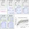
a) Stage 1: rats are trained only on the location task, with strong location evidence and no frequency evidence (pulses consist of superimposed low and high frequency). The context cue is played before each trial. b) Stage 2: rats learn to alternate between the location and frequency context. In the frequency context rats are presented with strong frequency evidence and no location evidence (stereo pulses). c) Stage 3: introduction of pulse modulation. In the frequency context, pulses are now presented on either side (but with no prevalent side). In the location context, pulses are either high-frequency or low-frequency (but with no prevalent frequency). d) Stage 4: irrelevant information is introduced, but the relevant information is always at maximum strength. e) Stage 5: relevant information can have intermediate strength. f) Stage 6: relevant information can have low strength. g) Training progression. Most rats learn stages 1-3 in approximately 2 weeks, but it takes a much longer time to learn stages 4-6 because of the introduction of irrelevant evidence. The feature selection index quantifies whether rats attend to the correct feature and ignore the irrelevant feature (see methods). The black dashed line indicates chance, the red dashed line indicates the threshold performance to consider a rat trained. Most rats learn the task within 2-5 months.

Extended Data Fig. 3. Behavioral data for all rats.

Rat ID color indicates whether rat was used for electrophysiology (red), optogenetics (cyan) or only for behavior (black). a) Psychometric curves for frequency evidence, measuring the fraction of right choices as a function of strength of frequency evidence (6 levels of strength, see Fig. 1b). Green indicates frequency context (relevant), purple indicates location context (irrelevant). b) Weights for frequency evidence computed using the behavioral logistic regression for each rat (see Fig. 1d); colors as in panel a. c) Differential behavioral kernel for frequency evidence across all rats. d) Psychometric curves for location evidence, measuring the fraction of right choices as a function of strength of location evidence (6 levels of strength, see Fig. 1b). Green indicates location context (relevant), purple indicates frequency context (irrelevant). e) Weights for location evidence computed using the behavioral logistic regression for each rat (see Fig. 1d); colors as in panel d. f) Differential behavioral kernel for location evidence across all rats. Shaded areas indicate bootstrapped standard errors. g) The slope index computed from behavioral trials in the first half split is highly correlated with the slope index computed using the second half split (r = 0.58; p = 0.000013). The significance of the correlation was computed using the Student’s t distribution. h) Psychometric curves can be predicted with high precision from the weights of the logistic regression. Data are shown from the seven rats used for electrophysiology recordings.

Extended Data Fig. 4. Electrophysiology and optogenetics techniques.

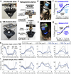
a) 64-channel custom-made multi-tetrode drive, allowing independent movement of 16 tetrodes. This drive was used in one rat for wired recordings. b) 128-channel custom-made multi-tetrode drive, allowing independent movement of 4 bundles with 8 tetrodes each. This drive was used in six rats for wireless recordings. c) Device for wireless optogenetic perturbation. In the implant, two chemically sharpened optic fibers targeting both hemispheres are attached using optical glue to two laser diodes. The laser diodes are controlled independently by a control board, which communicates wirelessly with the computer controlling the behavior. The control board can be attached/detached using a microUSB connector. d) Example rat with wireless electrophysiology implant and headstage. e) Example rat with wireless optogenetic implant and control board. f,g) Result of inactivation of FOF. 3 rats expressed AAV2/5-mDlx-ChR2-mCherry and were stimulated with blue light (450 nm, 25mW) for the full duration of the stimulus. f) Result of unilateral inactivation on rats’ choices as a function of strength of relevant evidence (averaged across the two contexts). Activation of each laser was randomized across trials. g) Result of bilateral FOF inactivation on rats’ choices as a function of strength of relevant evidence (averaged across the two contexts). h,i) Example responses of single units recorded in FOF (h) and in mPFC (i). Shown are the peri-stimulus time histograms of responses for correct trials, averaged according to context and choice. Units in both areas exhibit significant heterogeneity and large modulation according to combinations of the rat’s upcoming choice and the current context. The dashed vertical lines indicate the beginning of the pulse-train stimulus presentation, the end of the pulse-train stimulus presentation, and the average time when the rat performed a poke in one of the two side ports to indicate his choice. Shaded areas indicate standard errors.

Extended Data Fig. 5. Choice-related dynamics, computed independently for each rat, and across the two contexts.

For each rat, the horizontal and vertical axes in the two subpanels are the same across the two panels, and are computed using data from both contexts. In panels a-g, the dynamics in each context are computed using the choice kernels of the pulse-based regression (see Fig. 1.1 in Extended Discussion). The kernels provide a regularized, noise-reduced version of the raw trajectories (which are shown for Rat 1 in panel h). The black dot indicates the time of the start of stimulus presentation (t = 0), the purple dots indicate the end of stimulus presentation (t = 1.3s). The line indicates the choice axis computed in the given context, and above the panels is indicated the angle between the choice axes computed across the two contexts.

Extended Data Fig. 6. Engineered recurrent neural networks (RNNs) across the entire solution space (Fig. 2g) all qualitatively reproduce rat TDR trial-based dynamics, but are distinguished by pulse-based analysis.

a) Architecture of the RNNs. (b) TDR analysis (orange frame) and pulse-based analysis (purple frame) applied to RNNs generated to span different points within the solution space, as indicated by the RNN symbol on the barycentric coordinates. The TDR analysis and the pulse-based analysis of one RNN at each position are shown, connected to their RNN position by the arrow. For the position at the very center of the triangle, three different RNNs at that position, trained by starting from different random initial weights, are shown. All RNNs qualitatively reproduce rat TDR trial-based dynamics. The variability of trial-based TDR seen across RNNs is not predictive of the position within the solution space, and even RNNs generated from the same point can produce variable TDR trajectories. In contrast, the estimated pulse-triggered response reliably indicates the position of RNNs along the vertical axis of the solution space.

Extended Data Fig. 7. Validation of pulse regression method.

a) Example application of the pulse regression to one example recorded unit. (b) Fraction of explained variance as a function of firing rate across all recorded units. (c,d) The pulse-regression kernels provide an accurate estimate of the response to a single isolated pulse. In (c) are shown the responses to a single isolated pulse of either location or frequency evidence in both contexts for an example RNN unit. In (d) are shown the estimates of these pulses from the dynamics of the RNN solving the task with regular trials featuring many consecutive pulses presented at 40 Hz. (e) Comparison of the direction of the true line attractor (computed by finding the RNN’s fixed points, see methods) with the choice axis estimated by the trial-based regression (Fig. 1f,g) and the pulse-based regression (Fig. 3). The choice axis closely approximates the direction of the true line attractor. (f) Kernels estimated using the assumption of gaussian noise closely approximate those estimated using the assumption of Poisson noise. Kernels are shown here for one example neuron. (g) Prediction accuracy does not improve when two separate kernels are computed for the early portion of the stimulus and the late portion of the stimulus. Here is shown the improvement in cross-validated prediction accuracy across all recorded neurons when using two separate kernels as compared to using a single kernel throughout the stimulus. The significance was evaluated using a two-tailed paired-sample t-test (p > 0.1). (h) Population pulse responses for two example rats, and corresponding differential pulse-triggered kernels for the 10 individual neurons with largest contributions to the choice axis.

Extended Data Fig. 8. Differential pulse responses and behavioral kernels.

a) Differential pulse responses across the RNNs shown in Fig. 5c. The number above each behavioral kernel indicates the fraction of direct input modulation for the associated RNN (same notation as in Extended Data Fig. 6). (b) Corresponding behavioral kernel for each RNN. (c) Differential pulse responses across all rats shown in Fig. 5d (n = 7 rats, two features per rat). Gray indicates location feature, blue indicates frequency feature. (d) Corresponding behavioral kernels for each rat and feature. Shaded areas indicate bootstrapped standard errors.

Extended Data Fig. 9. Three distinct “languages” can capture the three fundamental solutions to the task.

a) “Linear algebra language”. As derived in the main text in Equations 1 and 2, the overall differential integration can be expressed as a sum of three terms. (b) “Network dynamics language”. The three solutions are associated with distinct pulse-evoked dynamics within the space spanned by the line attractor and the selection vector. (c) “Circuit dynamics language”. The three solutions are associated with three different latent circuit structures. To show this, we first note that our derivation of task solutions stems from focusing on linearized dynamics around fixed points of a line attractor (Fig. 2c). These linearized dynamics can be interpreted as an equivalent linear circuit whose synaptic connectivity matrix is defined by the state transition matrix (i.e. matrix M in Equation (1)). This circuit can be further simplified into a feedforward circuit using the Schur transformation (Goldman, 2009), which operates a change of coordinates to transform the state transition into an upper triangular form. In the resulting circuit, the first node represents the accumulator (i.e. the line attractor), and it receives feed-forward inputs from the other nodes of the circuit. Our three solutions can be interpreted as three different ways to modulate the connectivity of this circuit across the two contexts. In the case of “direct input modulation”, it is the input to the accumulator node that varies across contexts. In the case of “indirect input modulation”, it is the input to the other nodes that changes across contexts, and this differential input eventually reaches the accumulator through the feed-forward connections. Finally, in the case of “selection vector modulation”, the input to all nodes stays the same across contexts, but the feed-forward connections between the other nodes and the accumulator node change across contexts.

Extended Data Fig. 10. Extension of the theory to the general case with context-dependent line attractors.

a) Rewriting of the equation describing the differential integration of a pulse across contexts (Equation 1) after the assumption that the line attractor is parallel across the two contexts is dropped. In this equation, the first three terms correspond to the same terms as in Equation 2, with addition of a fourth term, which captures changes in the direction of the line attractor along the average input direction. (b) Graphical intuition of the four solutions in the general case where the line attractor is not parallel across the two contexts. Top left: changes of the input along the direction of the line attractor (“direct input modulation”). Top right: changes of the input along a direction orthogonal to the line attractor (“indirect input modulation”). Bottom left: changes of the direction of the line attractor across the two contexts. Bottom right: changes of the component of the selection vector orthogonal to the line attractor across contexts (“selection vector modulation”).

References

1. Okazawa, G. & Kiani, R. Neural mechanisms that make perceptual decisions flexible. Annu. Rev. Physiol. 10.1146/annurev-physiol-031722-024731 (2022). - PMC - PubMed
1. Livneh, Y. et al. Homeostatic circuits selectively gate food cue responses in insular cortex. Nature546, 611–616 (2017). - PMC - PubMed
1. Sarel, A. et al. Natural switches in behaviour rapidly modulate hippocampal coding. Nature609, 119–127 (2022). - PMC - PubMed
1. Mante, V., Sussillo, D., Shenoy, K. V. & Newsome, W. T. Context-dependent computation by recurrent dynamics in prefrontal cortex. Nature503, 78–84 (2013). - PMC - PubMed
1. Siegel, M., Buschman, T. J. & Miller, E. K. Cortical information flow during flexible sensorimotor decisions. Science348, 1352–1355 (2015). - PMC - PubMed