Effective data visualization strategies in untargeted metabolomics

Abstract

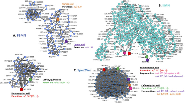
Covering: 2014 to 2023 for metabolomics, 2002 to 2023 for information visualizationLC-MS/MS-based untargeted metabolomics is a rapidly developing research field spawning increasing numbers of computational metabolomics tools assisting researchers with their complex data processing, analysis, and interpretation tasks. In this article, we review the entire untargeted metabolomics workflow from the perspective of information visualization, visual analytics and visual data integration. Data visualization is a crucial step at every stage of the metabolomics workflow, where it provides core components of data inspection, evaluation, and sharing capabilities. However, due to the large number of available data analysis tools and corresponding visualization components, it is hard for both users and developers to get an overview of what is already available and which tools are suitable for their analysis. In addition, there is little cross-pollination between the fields of data visualization and metabolomics, leaving visual tools to be designed in a secondary and mostly ad hoc fashion. With this review, we aim to bridge the gap between the fields of untargeted metabolomics and data visualization. First, we introduce data visualization to the untargeted metabolomics field as a topic worthy of its own dedicated research, and provide a primer on cutting-edge visualization research into data visualization for both researchers as well as developers active in metabolomics. We extend this primer with a discussion of best practices for data visualization as they have emerged from data visualization studies. Second, we provide a practical roadmap to the visual tool landscape and its use within the untargeted metabolomics field. Here, for several computational analysis stages within the untargeted metabolomics workflow, we provide an overview of commonly used visual strategies with practical examples. In this context, we will also outline promising areas for further research and development. We end the review with a set of recommendations for developers and users on how to make the best use of visualizations for more effective and transparent communication of results.

Fig. 1. Scatter plots of twelve of the thirteen datasaurus datasets (see ESI for X-shape variant). The datasaurus dataset is a constructed dataset intended to illustrate how misleading summary statistics and models outcomes can be, and how powerful visualization can be at showing the actual differences behind apparently similar overview statistics. Each dataset is constructed in such a way that summary statistics match those of a Dinosaur scatter plot drawing. Specifically, each dataset has near identical X and Y variable means and standard deviations, near identical correlation between X and Y variables, and, a linear model fitted to model Y as a function of X in each case has near identical intercepts and slope, as well as identical R squared summary statistics. This makes the datasets indistinguishable from the perspective of a comprehensive set of summary statistics. Visual inspection of the tables is also insufficient to grasp differences in the data. In the figure above, X and Y axes for all plots are identical and range from 0 to 100. Axis labels and tick marks are not shown as they are not essential.

Fig. 2. Overview of the untargeted metabolomics workflow. Color-highlighted nodes represent the data analysis stages and their visual components covered by this review. Analyses in untargeted metabolomics rarely follow a strict linear path, with different stages of the analyses happening in different order or not at all depending on the study. Central to all stages are stage-specific or inter-stage analysis and presentation visualizations.

Fig. 3. This review is situated in the intersection between the metabolomics researcher perspective, the metabolomics developer perspective, and the visualization field experts perspective. In particular, we aim to provide researchers with an overview of the visual capabilities available to them, provide developers with an overview of what possibilities and uncovered needs are, and visualization experts with an entry point to the current state of visualization in metabolomics. A primary aim of this review is to raise awareness of potential cross pollination of the visualization field into untargeted metabolomics. Rather than being comprehensive, we intend to provide an overview and highlight hot topics and refer to more focused reviews for details.

Fig. 4. The visual analytics pipeline of Keim et al.

Fig. 5. Brehmer and Munzner's visualization “How's” of designing visual idioms, i.e., “Encode”, “Manipulate”, “Facet”, “Reduce”, and “Introduce”, each of which features two to three lower-level approaches thereto. Encode describes how data is visually represented and presented to the user. Its two constituent approaches, i.e., “arrange” and “map”, are simply two examples of a much larger, exhaustive set discussed by Munzner. Manipulate describes different approaches to interactively altering the visual representation, such as, within the context of network visualization, “changing” the layout of a graph by clicking and dragging nodes, “selecting” groups of nodes to highlight them, or “navigating” through a visualization through zooming and panning. Facet describes the act of viewing different aspects of the same dataset or viewing the same dataset in a different way. “Juxtapositioning”, for example, is the process of breaking one view into multiple views based on some categorical variable. “Partitioning” describes breaking up one view into multiple based on some (user-defined) point along some variable. Lastly, “superimposition” is the opposite of juxtapositioning, i.e., bringing two separate views of the data together into a single one. Reduce is simply the process of reducing the visual complexity presented. In its simplest form, this takes the form of “filtering”, i.e., the removal of data not currently of interest. “Aggregation” is the creation of visual summaries of data points, e.g., the grouping of two or more bars of a bar chart into a single bar. More complex, “embedding” describes summarizing all data points into some form of visual abstraction, e.g. individual bar charts into a list of glyphs. Finally, Introduce is the introduction of new visual elements or data to an existing visualization, such as “annotating” a node's attributes in a node-link diagram, “importing” another (sub)graph alongside some already embedded one, or “deriving” a new data element based on existing data.

Fig. 6. Brehmer and Munzner's visualization “Why's” underlying the use of visualization, i.e., why a particular task is performed. Here, the authors identify four broader goals, comprised of higher levels ones, i.e., “Consume” and “Produce”, mid-level goals, i.e., “Search”, and low-level goals, i.e., “Query”. Each of these bigger-picture goals is additionally broken down further into three to four categories. First, consume describes the common uses of visualizations by domain experts and lay people. This includes “discovering” novel aspects about their data, such as validating or generating novel hypotheses, “presenting” data in a targeted manner to others, or merely “enjoying” a visual representation casually. Produce is the creation of novel “artifacts”, such as adding “annotations” to a dataset, “recording” new (visual) data, such as an ongoing time-dependent process, or “deriving”. Searching, as the name implies, is the process of locating particular data of interest. Depending on whether the data itself and its location in the visualization is known a priori, this process is either described as “exploring” (both target and location unknown), “browsing” (location known, target unknown), “locating”, (location unknown, but target known) or “looking up” (both target and location known). Finally, query describes the low-level processes a user aims to complete once their target(s) have been located; “identification” is the process of returning characteristics of particular data, “comparison” is the visual comparison of data characteristics, and “summarization” is the process of aggregating characteristics of the target data.

Fig. 7. Presentation of the effectiveness of different visual channels for communicating variable magnitude, ordered according to Munzner's effectiveness ranking from left to right, row by row. More specifically, in order of effectiveness: positions on a common scale, positions on an uncommon scale, angle, 2D length, 2D area, 3D depth, color luminance, color saturation, 2D curvature, and 3D volume.

Fig. 8. Illustration of the effectiveness of different visual channels to communicate magnitude. Here, across five hypothetical points in time, the magnitude of an imaginary variable has been recorded for two separate groups, colored orange and blue, respectively. In accordance with the ranking of visual channels presented in Fig. 7, the differences between these groups, as well as the overall trend of the data, is understood best when presented as positions on a common scale. Less effective is reliance on each bar's length to communicate differences. The least effective, at least for the example presented here, is the use of color saturation.

Fig. 9. Presentation of the effectiveness of different visual channels for communicating variable identity, ranked from left to right. More specifically, from most to least effective: region, color hue, motion, and finally shape.

Fig. 10. Illustrative representations of the here-discussed abstract graph layout approaches, i.e. straight-line node-link diagrams, radial node-link diagrams, layered node-link diagrams, schematic node-link diagrams, adjacency matrices, and hybrid approaches. All six representations utilize the same graph G = (V, E), where V = {A, B, C, D, E, F, G, H, I, J, K}, with the same |E| = 16 undirected edges between them.

Fig. 11. Commonly used visualization during raw data processing & spectral comparison. (A) Chromatogram. (B) Spectrum on MS level. (C) Fragmentation spectrum on MS/MS level. (D) Total Ion count for each sample, colors could be indicative of treatment. (E) Detected peaks for retention time and m/z. (F) Detected peaks for retention time and m/z including their intensity. (G) Deconvolution. (H) Alignment of one peak across different samples after retention time correction; color could be indicative of treatment. (I) Retention time correction amount. Usually plotted with retention time being on x-axis and the deviation after retention time correction on the y-axis. (J) Fragmentation spectrum of a target metabolite compared to a reference metabolite. (K) Fragmentation spectrum of a target metabolite next to a reference metabolite. (L) Fragmentation spectrum of a target metabolite with fragmentation of reference metabolite subtracted. (M) Fragmentation spectrum of a target metabolite compared to a reference metabolite with differences highlighted, while exact matches are faded. (N) Fragmentation spectrum of a target metabolite compared to a reference metabolite including hybrid search. (O) PCA plot with individual data points highlighted according to treatment. Abbreviation used in figure: m/z = mass to charge ratio, PCA = Principal component analysis. RT = retention time.

Fig. 12. Example screenshots of selected software in metabolomics raw data processing for each step. The typical steps of metabolomics raw data processing start with the initial raw data inspection, followed by peak detection, deconvolution, alignments and retention time (RT) correction, gap filling, and final visualization after processing (left column). MZmine (A–F) and XCMS (R version; G–L) have visualization throughout all the steps, while TOPPView (M) and MS-DIAL have a raw data viewer (N). MS-DIAL exclusively has a final post-processing viewer (O). (A) MS fragmentation spectrum of raw data. (B) MS fragmentation spectrum after peak detection, 3D plot of RT vs. m/z vs. intensity, and peak table showing the peak shape for every feature. (C) Deconvolution as differently colored peaks in chromatogram. (D) Peak table after RT alignment showing in which samples the peak has been found (green dot) and in which ones not (red dot). (E) Peak table after gap filling. Red dots turn yellow if peaks are now included. (F) Final visualization after processing raw data. Individual windows show peak shapes, MS/MS fragmentation spectrum, chromatograms of multiple samples, scatter plot of peak areas of two samples, 2D and 3D plot of a peak (RT vs. m/z vs. intensity), and line graph of peak over multiple samples (*Screenshot taken from MZmine2 (ref. 176)). (G) Chromatograms of each sample and total ion counts, both colored based on treatment. Additionally shown correlation heatmap for the samples based on raw data only. (H) Heatmap with binned retention time on the x-axis and samples on the y-axis showing the number of detected peaks and a 2D scatter plot of identified peaks (retention time against mass-to-charge ratio per sample). (I) Deconvolution shown with line drawn between individual peaks in chromatogram. (J) Retention-time-correction line plot and chromatographic test-peak before and after alignment. (K) Table showing the amount of missing peaks before and after gap filling. (L) Bi-plot from principal component analysis. (M) Raw data viewer of TOPPView. Upper panel shows MS view (RT by m/z); each box is a peak with color giving indication of peak intensity, while the lower panel shows the MS/MS fragmentation spectrum. (N) Raw data viewer of MS-DIAL show bar graphs for RT, MS and MS/MS spectrum intensity. (O) Final visualization of MS-DIAL after processing including MS spectrum, Retracted ion chromatogram, Meta data, peakspot viewer, and mirror plot.

Fig. 13. Spectral comparison plots usually portray two MS/MS fragmentation spectra via their mass-to-charge ratios and normalized intensities. The aims of pairwise spectral comparisons are (i) to assess library match quality, and (ii) to gain structural hypotheses within annotation propagation endeavors. From a visualization perspective, spectral comparison plots employ a wide variety of lower level “how's”. Specifically, they make use of (i) Encode → Arrange, displaying spectra by mass-to-charge ratio, (ii) Introduce → Annotate, where mass fragments may be automatically or manually annotated with chemical formulas, (iii) Facet → juxtapose/superimpose, where the two spectra are shown either side by side, in inverted y-axis, or contrasted to one another via subtractive approaches, (iv) Manipulate → Select, where additional fragment specific metadata such as precise mass to charge ratios or auto-generated chemical formulas may be viewed via hover tooltips, (v) Manipulate → Navigate, where zooming and panning allows for viewing areas of the spectra in more detail. The low level goals of the comparative plots are (i) Query → Compare, for the comparison of the spectra, (ii) Consume → Present, to present the mass spectral data, (iii) Produce → Annotate, where the user wants to gain insights into fragments and their likely chemical identity, and (iv) Search → Explore, where the user starts the spectral comparison with little knowledge of the fragmentation or characteristic fragment ions of both spectra. Spectral comparison plots thus provide a myriad of functions and encodings that assist data analysis well beyond spectral similarity scores.

Fig. 14. Mass spectral networks serve a wide variety of functions in the exploratory analysis of untargeted metabolomics data. The three main higher-level functions of molecular networking are (i) mass spectral data organization via the subdivision into molecular families, (ii) data exploration via interactive inspection of features and their interconnectivity, and (iii) as a data integration scaffold for analysis and presentation. Many different technical “how's” are used to make molecular networking as versatile as it is, including (i) Encode → Arrange, where MS/MS spectral features are arranged into node-link diagrams by cluster size, or in more recent developments overlaid onto a latent variable space, (ii) Reduce → Filter, where connectivity between features is limited via spectral similarity and topological constraints, (iii) Reduce → Embed, where mass spectral features are represented by node glyphs or more complex representations encoding additional information, (iv) Manipulate → Select, where hover information is used to provide node information, (v) Manipulate → Navigate, where panning and zooming is used to inspect broad areas or focus in on local areas, (vi) Introduce → Annotate, where additional spectral annotation information or library matches are introduced for nodes, and (vii) Introduce → Import, where statistical information, annotations, or experimental information can be included as color, size, glyph, or shade information. From a visualization perspective, the goals of molecular networking fall into the categories of (i) Produce → Annotate, where features and clusters of features are annotated, (ii) Produce → Derive, where node link diagrams are derived from spectral similarity data, (iii) Search → Explore, where nodes of interested are sought for inside node-link diagrams via their connectivity or annotations, (iv) Query → Identify, where once a node of interest is found, it's annotation and available information are sought for, and (v) Query → Compare, where spectral features are compared beyond the thresholded pairwise similarity-based edges. With such a variety of technical components and goals, it is no surprise that molecular networking is commonly used, used for different purposes, and modified into different workflows that facilitate particular analysis tasks in a more targeted fashion.

Fig. 15. Example molecular networking families for ESI-negative MS/MS spectral datasets from maize leave samples (see also ESI†). Figures show sub-networks for (A) feature-based molecular networking (FBMN), (B) ion identity molecular networking (IIMN) and (C) Spec2Vec similarity-based networking generated from samples. The different figures reveal differences in the clustering of related ion species when different molecular networking approaches or similarity scoring methods are applied. The example data are from ongoing research on maize samples. Here, the highlighted compound structures are library hits for hydroxycinnamic acid (HCA) compounds of interest. Initial FBMN revealed high numbers of in-source fragmentation and separation of parent ions from the HCA compound class of interest which were expected to cluster together. Subsequent analysis using IIMN tackled the in-source fragment redundancy and the use of the Spec2Vec similarity score improved the clustering of the HCA features into one densely connected network. The complexity of the visual analytics process underlying the use of molecular networking is striking in this example, where different variants of molecular networking are iteratively applied to improve data organization within an overarching effort to make use of library matches to explore and annotate additional features.

Fig. 16. Representation of different means of representing mass spectral similarity data. (A) Similarity data are subjected to topological filtering and represented as (disconnected) node-link-diagrams (e.g. molecular networking). (B) Similarity data are subjected to a two-dimensional embedding algorithm projecting them onto a two-dimensional plane, and represented using a scatter plot (e.g., MetGem and specXplore). (C) Interactive node-centric neighborhood displays using top-k edges for the selected node are added as an overlay to the embedding representation. This affords insights into connectivity beyond the embedding projection, and with adjustable top-k values, allows fluid exploration of intra- and inter-cluster connectivity (e.g. msFeaST). (D) Edge overlays at specific threshold levels for clusters of features can pinpoint inter-cluster connectivity via the two-dimensional embedding projection (e.g., specXplore).

Fig. 17. An example of a molecular networking infographic that uses pie charts to highlight differences in intensity of precursor ions of metabolites that are observed among sample groups. In addition to pie charts, network properties such as node color or size can be mapped to relevant variables to help differentiate the most relevant nodes. Putative identities of the features are provided with the name and structure of spectral library matches, m/z of the feature is shown below the node. Here, rectangular nodes represent individual metabolite features, the size of the nodes represents total feature abundance, and node colors indicate where the feature is detected (MS = mushroom substrate, FB = fruiting body, and SMS = spent mushroom substrate). The pie charts show proportions of feature abundance for samples with different concentrations of olive mill solid waste. Through Zenodo, an R script is available together with the example input data and expected output data that automates network processing and annotation, creating network visualizations such as the one shown here (https://zenodo.org/doi/10.5281/zenodo.12756070) Data was used from (ref. 219) – see also ESI.

Fig. 18. Volcano plots portray statistical summary data of repeated univariate tests on each feature, providing the user with a means of obtaining (a) an overview of the experimental impact on intensity profiles, and (b) a means of sub-selecting features with statistical differentiation across treatment groups. On a technical level, the lower level “how's” of the volcano plot are (i) Endode → Arrange, where p-values and fold changes are arranged by their magnitude, (ii) Encode → Map, where statistical significance and substantive effects are mapped to color/glyph/shade of points, and (iii) Reduce → Filter, in that features of statistical or substantive effect are emphasized over condensed areas of features of lesser effect. To a more limited extend, Manipulate → Navigate is used to allow inspection of crowded areas via panning and zooming. From a visualization perspective, the main lower level goals of volcano plots are (i) Query → Summarize, where intensity summary data are summarized using statistical measures, (ii) Consume → Present, where the plot provides an overview of the general trends across conditions, (iii) Search → Locate, where users can locate and identify features of interest via their position in the plot. Applying to a lesser extend is Search → Look-up, where users may want to assess known features of interest within the plot. Volcano plots are thus a prime example of Shneiderman's “Overview first, zoom and filter, then details-on-demand”. In applied analyses, they could be fruitfully combined with follow-up visualization or analyses in a myriad of ways, including the generation of promising subselections for in-depth visualization in heatmaps, or the highlighting of promising subselections in mass spectral similarity networks.

Fig. 19. Example of a knowledge graph network integrating multiple omics data layers. Nodes are categorized and color-coded as follows: blue nodes represent ontology terms related to experimental design (e.g., sample_id_X, time_point), phenotype, genomics (e.g., genome_X, gene_X), and metabolomics (e.g., feature_list, chemical_class). Orange nodes denote ontology terms for methods and analytical tools (e.g., Library matching, ClusterONE). Purple nodes correspond to databases and other data sources (e.g., Zenodo, NCBI). Edges between nodes represent relationships via ontology terms, facilitating the extraction and standardization of information across the graph.

Kevin Mildau

Henry Ehlers

Fidele Tugizimana

Florian Huber

Justin J. J. van der Hooft

References

1. Munzner T., Visualization Analysis and Design, CRC Press, 2014
1. Matejka J. and Fitzmaurice G., Proceedings of the 2017 CHI Conference on Human Factors in Computing Systems, 2017
1. Murray L. L. Wilson J. G. Decis. Sci. J. Innov. Educ. 2021;19:157–166.
1. Andrienko N., Andrienko G., Fuchs G., Slingsby A., Turkay C. and Wrobel S., in Visual Analytics for Investigating and Processing Data, Springer International Publishing, 2020, pp. 151–180
1. Liu S. Cui W. Wu Y. Liu M. Vis. Comput. 2014;30:1373–1393. doi: 10.1007/s00371-013-0892-3. - DOI
Publication types
LinkOut - more resources