Membrane mechanics dictate axonal pearls-on-a-string morphology and function

Abstract

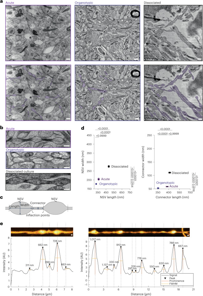
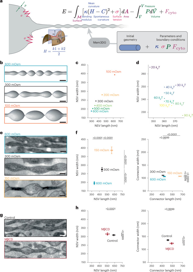
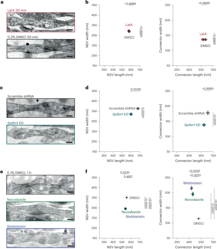
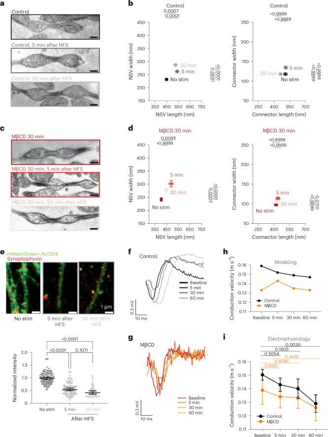
Axons are ultrathin membrane cables that are specialized for the conduction of action potentials. Although their diameter is variable along their length, how their morphology is determined is unclear. Here, we demonstrate that unmyelinated axons of the mouse central nervous system have nonsynaptic, nanoscopic varicosities ~200 nm in diameter repeatedly along their length interspersed with a thin cable ~60 nm in diameter like pearls-on-a-string. In silico modeling suggests that this axon nanopearling can be explained by membrane mechanical properties. Treatments disrupting membrane properties, such as hyper- or hypotonic solutions, cholesterol removal and nonmuscle myosin II inhibition, alter axon nanopearling, confirming the role of membrane mechanics in determining axon morphology. Furthermore, neuronal activity modulates plasma membrane cholesterol concentration, leading to changes in axon nanopearls and causing slowing of action potential conduction velocity. These data reveal that biophysical forces dictate axon morphology and function, and modulation of membrane mechanics likely underlies unmyelinated axonal plasticity.

Fig. 1. Axons are pearled, not tubular, under homeostatic conditions.

a, Representative electron micrographs from acutely extracted mouse brain tissue (left), organotypic slice cultures of mouse hippocampus (middle) and dissociated mouse hippocampal neuronal culture after high-pressure freezing. Some axons in each micrograph are traced and color coded on the bottom; scale bars, 500 nm. b, High-magnification images of axons representative of each condition. More example micrographs are found in Extended Data Fig. 1a,b,e; scale bars, 200 nm. c, A schematic showing two NSVs flanked by a connector. Inflection points define the boundary between these two features. Both width and length are measured at NSVs and connectors, as shown. d, Plots showing dimensions of NSVs (left) and connectors (right) from indicated tissue types. Dimensions are measured from three independent samples for acutely extracted brain tissue and dissociated neuron culture and one for organotypic slices; n = 30 axons from each acutely extracted sample, n = 133 axons from the organotypic sample, and n = 100 axons from each dissociated sample. Super plots showing variability are available in Extended Data Fig. 1f. Data are shown as mean ± s.e.m. and were analyzed by Kruskal–Wallis test, followed by a Dunn’s multiple comparison test. e, Representative STED micrographs showing axons from organotypic slice cultures of mouse hippocampi. The numbers represent the length of each NSV, measured at full-width half-maximum (FWHM) using MATLAB scripts. Numbers indicate the measured length at each NSV; scale bars, 200 nm; AU, arbitrary units. Source data

Fig. 2. Membrane mechanics dictate axon nanopearling.

a, Axon morphology is modeled using the classic Helfrich membrane model and governed by membrane bending, surface tension and osmotic conditions. b, Model prediction of axon morphology under the indicated osmotic conditions; scale bars, 200 nm. c, Plot showing the dimensions of NSVs at the indicated osmotic conditions. Note that NSV size is inversely scaled with the external osmotic pressure. d, Plot showing the dimensions of NSVs with varying membrane rigidity, ranging from 20 k_BT to 100 k_BT. e, Example micrographs of axons high-pressure frozen under the indicated osmotic conditions. More example micrographs are available in Extended Data Fig. 3a; scale bars, 200 nm. f, Plots showing the dimensions of NSVs (left) and connectors (right) from neurons in e; n = 100 axons from three replicates. Super plots showing variability are available in Extended Data Fig. 3b. Data are shown as mean ± s.e.m. and were analyzed by Kruskal–Wallis test, followed by a Dunn’s multiple comparison test. g, Example micrographs of axons from cultured neurons treated with sham (control) or 5 mM MβCD for 30 min. More example micrographs are available in Extended Data Fig. 4c; scale bars, 200 nm. h, Plots showing the dimensions of NSVs (left) and connectors (right) from neurons in g; n = 100 axons from three replicates. Super plots showing variability are available in Extended Data Fig. 4d. Data are shown as mean ± s.e.m. and were analyzed by Kruskal–Wallis test, followed by a Dunn’s multiple comparison test. Source data

Fig. 3. MPS is not sufficient to explain pearled axon morphology.

a, Example micrographs of axons from cultured mouse hippocampal neurons treated with either 0.2% DMSO or 20 µM LatA for 30 min; scale bars, 200 nm. b, Plots showing the dimensions of NSVs (left) and connectors (right) from axons in a (DMSO: NSV length 630 ± 13 nm, NSV width 320 ± 5 nm, connector length 600 ± 18 nm, connector width 136 ± 3 nm; LatA: NSV length 230 ± 11 nm, NSV width 320 ± 5 nm, connector length 570 ± 20 nm, connector width 136 ± 4 nm). c, Example micrographs of axons from neurons infected with lentivirus carrying either scramble or Sptbn1 (βII spectrin) shRNA; scale bars, 200 nm. d, Plots showing dimensions of NSVs (left) and connectors (right) from axons in c. e, Example micrographs of axons from neurons treated with 0.1% DMSO, 50 µM nocodazole or 10 µM blebbistatin for 1 h; scale bars, 200 nm. f, Plots showing dimensions of NSVs (left) and connectors (right) from axons in e (DMSO: NSV length 600 ± 12 nm, NSV width 350 ± 7 nm, connector length 520 ± 19 nm, connector width 115 ± 3 nm; nocodazole: NSV length 590 ± 10 nm, NSV width 300 ± 3 nm, connector length 450 ± 13 nm, connector width 200 ± 6 nm; blebbistatin: NSV length 590 ± 11 nm, NSV width 290 ± 4 nm, connector length 430 ± 12 nm, connector width 215 ± 5 nm). In each experiment, N = 3 independent cultures and n = 300 axons. Super plots showing variability are available in Extended Data Fig. 5. Data are shown as mean ± s.e.m. All conditions in the figure were analyzed at the same time, and, thus, a Kruskal–Wallis test followed by a Dunn’s multiple comparison test was used. Source data

Fig. 4. AP propagation relies on axonal morphology.

a, Schematic showing the model setup. APs were modeled in real geometries using a generalized cable equation to calculate the spatial and temporal distribution of channel current, membrane voltage and gating variables. b, Voltage responses at 270 µm from cylindrical axons (left) and pearled axons (right) when NaVs are distributed either uniformly (dark color) or periodically (lighter color). Note that the distribution of NaVs only matters if axons are pearled. c, Plot of the relationship between AP velocity and the diameter of cylindrical axons. Dots are fitted with a simple linear regression curve. d–g, Plots of the relationship between AP velocity and the connector width (d), connector length (e), NSV width (f) and NSV length (g). Dots are fitted with a simple linear regression curve, except for f, which is fitted by a nonlinear Gaussian curve. h, Plot of predicted AP conduction velocity based on the dimensions of NSVs and connectors in neurons treated with sham (control) or 5 mM MβCD. i, Schematic of the electrophysiology recording setup. Schaffer collaterals were stimulated from the end of CA1 to measure the back-propagating AP in the CA1. j, Example traces from recordings in acute slices of mouse hippocampus treated with either sham (control) or 5 mM MβCD for 30 min. The solid vertical line marks the peak. k, Plot of AP conduction velocity from the experiments in j. Data were analyzed by Mann–Whitney U-test (two sided) and are shown as mean ± s.d.; N = 8 animals each, n = 14 slices for DMSO, and n = 12 slices for MβCD. Source data

Fig. 5. Axonal plasticity is mediated by modulation of membrane mechanics.

a, Example micrographs showing axon morphology from control neurons unstimulated or stimulated with three trains of 100 pulses at 100 Hz (HFS) and high-pressure frozen at 5 and 30 min after stimulation; scale bars, 200 nm. b, Plots showing the dimensions of NSVs (left) and connectors (right) from axons in a. Data are shown as mean ± s.e.m. and were analyzed by Kruskal–Wallis test, followed by a Dunn’s multiple comparison test; N = 3 independent cultures and n = 100 axons each. c, Example micrographs showing axon morphology from MꞵCD-treated neurons (5 mM for 30 min) unstimulated or stimulated with three trains of 100 pulses at 100 Hz (HFS) and high-pressure frozen at 5 and 30 min after stimulation; scale bars, 200 nm. d, Plots showing the dimensions of NSVs (left) and connectors (right) from axons in c. Data are shown as mean ± s.e.m. and were analyzed by Kruskal–Wallis test, followed by a Dunn’s multiple comparison test; N = 3 independent cultures and n = 100 axons each. e, Example images and plots showing normalized intensity of the cholesterol biosensor NeonGreen–ALOD4 in neurons unstimulated or stimulated with HFS and fixed 5 or 30 min after. Data are shown as median and 95% confidence interval (no stimulation (stim): 0.99, 95% confidence interval 0.95–1.04, n = 109; 5 min after HFS: 0.54, 95% confidence interval 0.52–0.61, n = 110; 30 min after HFS: 0.42, 95% confidence interval 0.44–0.54, n = 91); N = 3 independent cultures. Data were analyzed by Kruskal–Wallis test, followed by a Dunn’s multiple comparison test. f, Example traces from electrophysiology experiments, performed as described in Fig. 4i. g, Example traces from electrophysiology experiments in acute slices of mouse hippocampus, performed as described in Fig. 4i. h, Predicted AP conduction velocity based on the dimensions of NSVs and connectors before and 5, 30 and 60 min after HFS. i, Measured AP conduction velocity before and 5, 30 and 60 min after HFS. Data are shown as mean ± s.e.m. and were analyzed by Kolmogorov–Smirnov test between curves (P = 0.23) and Mann–Whitney U-test (two sided) between individual time points within treatment conditions. Source data

Extended Data Fig. 1. Pearled morphology is observed for all axons except after chemical fixation.

a. Example micrographs showing acutely extracted mouse brain tissue either high-pressure frozen (left) or chemically fixed (right). The boxed axons are reconstructed using IMOD. Note that chemically fixed axons are like cylindrical tubes. Scale bar: 500 nm. b. Higher magnification images of the boxed area in a. Scale bar: 200 nm. c. AiryScan images of axons live without (left) or after 5 min of fixation (right). Inset shows synapses marked by RIM1a-CFP. Arrowheads mark synapses, arrows mark NSVs, circle marks extreme axon pearling associated with degenerating axons. Scale bar: 5 µm. d. Further images of an axon from a separate culture live without (middle) or after 5 min of fixation (bottom). Synapses marked by RIM1a-CFP (top). Arrowheads mark synapses, arrows mark NSVs. Scale bar: 1 µm. e. Additional representative images of axons from acutely extracted brain tissue, organotypic slice culture, and dissociated neuron culture. Scale bar: 200 nm. f. Super Plots of Fig. 1d, showing experimental variability. Median and 95% confidence intervals are shown. N = 3 and n = 30 axons from each acutely extracted sample, n = 133 axons from the organotypic sample, N = 3 and n = 100 axons from each dissociated sample. Kruskal-Wallis test, followed by Dunn’s multiple comparison test was used. Each color represents one replicate. Each dot is one axon. g. Frequency distributions for acute, organotypic, and dissociated culture of either NSV lengths or connector lengths. h. Additional STED micrographs showing pearled axon morphology in live neurons from organotypic slice cultures. Scale bar: 500 nm. Individual axons are straightened and represented on the right panels. Scale bar: 200 nm. Source data

Extended Data Fig. 2. Manipulation of membrane mechanics predicts changes in axonal pearling.

a. Axon morphology is modeled using classic Helfrich membrane model and governed by the membrane bending, surface tension, and osmotic condition. 3D model prediction of axon morphology in indicated osmotic conditions, tension of 0.001 mN/m, and bending rigidity of 50kBT. Scale bar: 200 nm. b. 3D model prediction of axon morphology at indicated bending rigidity, tension of 0.001 mN/m, and osmolarity 300 mOsm. Scale bar: 200 nm. c. Rotationally averaged shape profiles of axons under constant 0.001 mN/m tension and varying osmotic conditions and bending rigidity. The bead diameter (D) and length (L) in nanometers are given as a text inset for each condition. d. Rotationally averaged shape profiles of axons under constant 0.01 mN/m tension and varying osmotic conditions and bending rigidity. The bead diameter (D) and length (L) in nanometers are given as a text inset for each condition. Source data

Extended Data Fig. 3. Manipulation of osmolarity causes changes in axonal pearling.

a. Additional example micrographs of axons high-pressure frozen at indicated osmotic conditions. Scale bar: 200 nm. b. Super Plots of Fig. 2f, showing experimental variability. c. Example micrographs of axons high-pressure frozen at indicated osmotic conditions. Mannitol was used to adjust the osmolarity. Scale bar: 200 nm. d. Super Plots of Extended Data Fig. 2e, showing the dimensions of NSVs at indicated osmotic conditions. e. Plot showing the dimensions of NSVs at indicated osmotic conditions. Mean and SEM are plotted. N = 3 independent cultures, n = 100 axons each. In all super plots median and 95% confidence intervals are shown. N = 3 independent cultures and n = 100 axons each. Each color represents one replicate. Each dot is one axon. All data analyzed using Kruskal-Wallis test, followed by Dunn’s multiple comparison test.

Extended Data Fig. 4. Manipulation of membrane cholesterol causes changes in axonal pearling.

a. NeonGreen-ALOD4 staining of cultured mouse hippocampal neurons treated with sham (control) or 5 mM MßCD for 30 min. Scale bar = 5 µm. b. Plot showing the normalized intensity of NeonGreen-ALOD4. Signals are normalized by the area of each region-of-interest. Control: 2773 ± 234 A.U., MβCD: 86 ± 13 A.U., median and 95% confidence intervals are plotted, Mann-Whitney U test (two-sided), N = 3 independent cultures, n = 127 for control, n = 131 for MβCD. A.U. arbitrary unit. c. Additional example micrographs of axons high-pressure frozen after MßCD treatment. Scale bar: 200 nm. d. Super Plots of Fig. 2h, showing variability. N = 3 independent cultures and n = 100 axons each. Median and 95% confidence intervals are plotted, Kruskal-Wallis test, followed by Dunn’s multiple comparison test. Each color represents one replicate. Each dot is one axon. Source data

Extended Data Fig. 5. Manipulation of the cytoskeleton causes changes in axonal pearling.

a. Western blots and quantification showing the efficiency of shRNA-mediated knock down (KD) of ßII spectrin magenta shows ßII spectrin and yellow shows GAPDH. Scr, scramble. b. Example micrographs of axons from neurons treated with indicated drugs. Scale bar: 200 nm. c. Plots showing dimensions of NSVs (left) and connectors (right) from axons in (a). Mean and SEM are shown. N = 3 independent cultures n = 100 axons each. n.s., not significant. d. Additional example micrographs of axons from neurons infected with lentivirus carrying scramble shRNA or shRNA against ßII spectrin. Scale bar: 200 nm. e. Super Plots of Fig. 3d, showing experimental variability N = 3 independent cultures and n = 100 axons each. f. Additional example micrographs of axons from neurons treated with indicated drugs. Note that these neurons are treated with DMSO or Latrunculin A for 1 hour. Scale bar: 200 nm. g. Super Plots, showing experimental variability of Fig. 3a. N = 1 and n = 100 axons. h. Additional example micrographs of axons from neurons treated with indicated drugs. Scale bar: 200 nm. i. Super Plots of Fig. 3f, showing experimental variability. N = 3 independent cultures and n = 100 axons each. j. Additional example micrographs of axons from neurons treated with indicated drugs. Scale bar: 200 nm. k. Super Plots, showing experimental variability from experiments in Extended Data Fig. 5j. N = 3 independent cultures and n = 100 axons each. In all super plots median and 95% confidence intervals are shown. Each color represents one replicate. Each dot is one axon. All data analyzed using Kruskal-Wallis test, followed by Dunn’s multiple comparison test. Source data

Extended Data Fig. 6. Live STED confirms LatA and CytoD, but not blebbistatin or nocodazole, disrupt actin ring organization.

a–g. Representative 2D STED images of live axon stained by SiR-actin under control (DMSO) or drug treatments with plotted intensity profile from region indicated by blue line and fast Fourier transform of intensity profile where the largest peak represents the most frequent distance between actin puncta. Histogram (black) and Gaussian distribution (red line) of actin puncta spacing from 50 axons in each condition from 2 independent cultures. a, DMSO control, Gaussian distribution values: avg. 245 nm S.D. 253 nm. b, LatA 30 min, Gaussian distribution values: avg. 352 nm S.D. 351 nm. c, DMSO control, Gaussian distribution values: avg. 235 nm S.D. 184 nm. d, LatA 1 hr, Gaussian distribution values: avg. 288 nm S.D. 265 nm. e, CytoD 1 hr, Gaussian distribution values: avg. 772 nm S.D. 482 nm. f, Blebbistatin 1 hr, Gaussian distribution values: avg. 152 nm S.D. 43 nm. g, Nocodazole 1 hr, Gaussian distribution values: avg. 174 nm S.D. 69 nm. Source data

Extended Data Fig. 7. AP velocity varies with axon pearl dimensions.

a-f, Plots showing the relationship between AP velocity and the ratio of two measured values like connector width/NSV width (a), connector width/NSV length (b), connector width/connector length (c), connector length/NSV length (d), NSV length/NSV width (e), and connector length/NSV width (f). The data are fitted by a simple linear regression in all except for e, which is fitted by a gaussian non-linear curve. g. Plot showing the predicted AP conduction velocity based on the dimensions of NSVs and connectors in neurons treated with sham (DMSO) or 50 µM Blebbistatin (bleb). h. Plot showing the AP conduction velocity from the experiments in (j). Mean and S.E.M. are plotted. Mann-Whitney U test (two-sided). N = 8 animals each, n = 12 slices. Source data

Extended Data Fig. 8. Axonal pearling changes with stimulation even after cholesterol manipulation.

a. Additional example micrographs showing axon morphology from neurons unstimulated or stimulated with 3 × 100 pulses at 100 Hz (high-frequency stimulation, HFS) and high-pressure frozen at 5 min and 30 min after stimulation. Scale bar: 200 nm. b. Super Plots of Fig. 5b, showing experimental variability. N = 3 independent cultures except for control 15’ post stim which was N = 2. n = 100 axons each. c. Super Plots of Fig. 5c, showing experimental variability. N = 3 independent cultures. n = 100 axons each. In all super plots median and 95% confidence intervals are shown. N = 3 independent cultures and n = 100 axons each. Each color represents one replicate. Each dot is one axon. All data analyzed using Kruskal-Wallis test, followed by Dunn’s multiple comparison test. Source data

References

1. Hodgkin, A. L. & Huxley, A. F. A quantitative description of membrane current and its application to conduction and excitation in nerve. J. Physiol.117, 500–544 (1952). - PMC - PubMed
1. Waxman, S. G. Determinants of conduction velocity in myelinated nerve fibers. Muscle Nerve3, 141–150 (1980). - PubMed
1. Acker, C. D. & White, J. A. Roles of IA and morphology in action potential propagation in CA1 pyramidal cell dendrites. J. Comput. Neurosci.23, 201–216 (2007). - PubMed
1. Zhou, Y. & Bell, J. Study of propagation along nonuniform excitable fibers. Math. Biosci.119, 169–203 (1994). - PubMed
1. Perge, J. A., Niven, J. E., Mugnaini, E., Balasubramanian, V. & Sterling, P. Why do axons differ in caliber? J. Neurosci.32, 626–638 (2012). - PMC - PubMed