Feature selectivity and invariance in marsupial primary visual cortex

Abstract

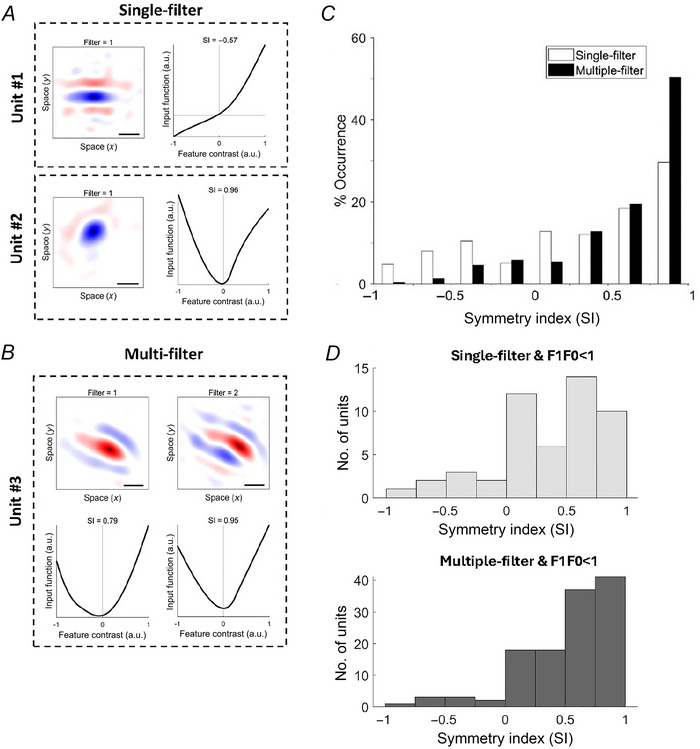
A fundamental question in sensory neuroscience revolves around how neurons represent complex visual stimuli. In mammalian primary visual cortex (V1), neurons decode intricate visual features to identify objects, with most being selective for edge orientation, but with half of those also developing invariance to edge position within their receptive fields. Position invariance allows cells to continue to code an edge even when it moves around. Combining feature selectivity and invariance is integral to successful object recognition. Considering the marsupial-eutherian divergence 160 million years ago, we explored whether feature selectivity and invariance was similar in marsupials and eutherians. We recovered the spatial filters and non-linear processing characteristics of the receptive fields of neurons in wallaby V1 and compared them with previous results from cat cortex. We stimulated the neurons in V1 with white Gaussian noise and analysed responses using the non-linear input model. Wallabies exhibit the same high percentage of orientation selective neurons as cats. However, in wallabies we observed a notably higher prevalence of neurons with three or more filters compared to cats. We show that having three or more filters substantially increases phase invariance in the V1s of both species, but that wallaby V1 accentuates this feature, suggesting that the species condenses more processing into the earliest cortical stage. These findings suggest that evolution has led to more than one solution to the problem of creating complex visual processing strategies. KEY POINTS: Previous studies have shown that the primary visual cortex (V1) in mammals is essential for processing complex visual stimuli, with neurons displaying selectivity for edge orientation and position. This research explores whether the visual processing mechanisms in marsupials, such as wallabies, are similar to those in eutherian mammals (e.g. cats). The study found that wallabies have a higher prevalence of neurons with multiple spatial filters in V1, indicating more complex visual processing. Using a non-linear input model, we demonstrated that neurons with three or more filters increase phase invariance. These findings suggest that marsupials and eutherian mammals have evolved similar strategies for visual processing, but marsupials have condensed more capacity to build phase invariance into the first step in the cortical pathway.

Keywords: brain evolution; marsupial; neuroscience; receptive field; visual cortex.

Figure 1. A simplified mammalian phylogenetic tree

The tree includes most of the species that have had their V1s studied using electrophysiology and (in some cases) imaging. MYA: millions of years ago. Images of brains are from the University of Wisconsin and Michigan State Comparative Mammalian Brain Collections (www.brainmuseum.org). If mammals in a particular phylogenetic line have pinwheel‐like orientation preference maps, pinwheels are shown in small boxes; if they have salt‐and‐pepper maps, random dot patterns are shown; if imaging has not been conducted, a question mark is shown. From left to right, the species are: opossum, possum, wallaby, sheep, cat, tree shrew, macaque, mouse, rat and rabbit. [Colour figure can be viewed at wileyonlinelibrary.com]

Figure 2. Schematic diagram of the NIM

In parallel streams: (1) visual stimulus is processed by several spatial filters, (2) the signal is then fed into the input non‐linearity, (3) the parallel streams combine together to produce a generator signal, (4) the generator signal is processed by the spiking non‐linearity and (5) the signal is randomized by a Poisson process to produce a spiking response for the neuron. [Colour figure can be viewed at wileyonlinelibrary.com]

Figure 3. Spatial receptive fields in V1

A, 10 example units are presented in rows, labelled 1–10, and the filter types are laid out in columns, labelled Filters 1–5. The estimated RF filters are all spatially localized. Within the spatial RFs, red regions represent the ON‐response subfields (i.e. responding to brightness increments) and blue regions represent the OFF‐response subfields (i.e. responding to brightness decrements). The size of RFs is indicated by the scale bar, which represents 1° in visual space. OB = orientation bias. An OB index of 0 is a unit responding equally to all orientations, while an OB index of 1 is a unit responding only to a particular orientation. B, the distribution of single‐ and multi‐filter units in the wallaby unit population. C, F1/F0 ratios for wallaby V1 units (n = 195). Grey and black columns represent simple and complex cells, respectively. The cells are binned into 0.1 bar widths. Cells with F1/F0 ratios > 2.2 are all presented to the far‐right bar. The distribution of simple and complex cells was significantly different from unimodality (Hartigan's dip statistic: P = 0.03). D, bar graph showing the distribution of the number of RF filters obtained from the NIM for classical simple and complex cells. Note that many simple cells had only a single filter and many complex cells varied from one to five filters when assessed using the NIM. [Colour figure can be viewed at wileyonlinelibrary.com]

Figure 4. Orientation selectivity of V1 units

A, histogram showing the distribution of OB values of all 195 single units recorded. Red dashed line indicates the threshold (OB = 0.2) between non‐oriented and oriented types. Of all the units recorded, 76% (n = 148/195) were oriented and 24% (n = 47/195) were non‐oriented. B, example RFs of single‐filter units with different OB values. C, histograms showing the OB indices for single‐filter, double‐filter and ≥3‐filter units. Orange bars are non‐oriented units; blue bars are orientation‐selective units. Numbers with arrows above each plot show the mean non‐oriented and oriented OB indices. [Colour figure can be viewed at wileyonlinelibrary.com]

Figure 5. Non‐linear properties of V1 units

Three example units with their RFs and corresponding input functions from the NIM. The red regions are ON responses and blue regions are OFF responses, in x and y space. The black bar indicates 1° in visual space. On the right side of the filters are the respective input non‐linearities plotted as input functions over feature contrast (arbitrary units: a.u.), and the grey lines represent the origin (x = 0, y = 0). The titles for the input function plots show the symmetry index (SI). A, top panel: single‐filter unit with an odd symmetric input function (SI = −0.57). Bottom panel: single‐filter unit with an even symmetric input function (SI = 0.96). B, multi‐filter unit with two spatial filters that have approximately even‐symmetric input functions (SI = 0.79, SI = 0.95). C, distributions of the SI of identified input functions for single‐filter (white bars) and multi‐filter cells (black bars). D, distribution of the SI values of identified input functions for single‐filter and multi‐filter cells with F1/F0 ratio < 1 (classically defined as complex cells). [Colour figure can be viewed at wileyonlinelibrary.com]

Figure 6. Selectivity and invariance in wallaby V1 cell

A, an example model fit #1 for a cell with spatial phase invariance (for the example 1 cell, the estimated input non‐linearities for both filters are close to quadratic). For this cell, the spectrum of interpolated features producing equal responses spans 2π radians of feature‐phase due to the closed elliptical isoresponse contours. The example cell is invariant to spatial phase because it responds equally to interpolated features that are spanning the full 360° of spatial phase. B, an example model fit #2 for a cell with two not even‐symmetric input functions. As a result of the openness of the isoresponse contours for this cell, the relative feature‐contrast varies significantly. For each example, two spatial RF filters (Filter 1 and Filter 2), derived from a WGN stimulus region, are shown on the top right. The two‐dimensional feature subspace plot shows the mean spike rates, represented by various shades of grey, in response to each interpolated feature embedded in WGN. Magenta isoresponse contours indicate equal spike rates for various feature‐phases and contrasts. Green dots represent a selection of interpolated features, each associated with specific coordinates within the feature subspace. Non‐linearities for these filters are represented by black curves over grey bar‐graphs, depicting cell responses across the WGN stimuli in feature space. B and E, feature‐contrast of interpolated features along isoresponse contours is plotted against feature‐phase, averaged across different spike rates. C and F, the features interpolated (i.e. orientation, spatial frequency, spatial phase) at different feature‐phases are sampled from an isoresponse contour within the cell's feature spectrum. The degree of variation observed in each feature characteristic is normalized relative to its inherent range of variation. [Colour figure can be viewed at wileyonlinelibrary.com]

Figure 7. Enhancing feature selectivity or invariance in wallaby V1 cells

Bar graphs illustrate the tuning widths of wallaby V1 cells categorized into three groups: those with two filters (left column), those with three filters (middle column), and those with four and five filters (right column). This analysis is presented across three fundamental feature attributes: (A) orientation, (B) spatial frequency and (C) spatial phase. Each vertical tick mark along the x‐axis represents an individual cell. The length of each thick black bar corresponds to the tuning width of the respective cell. Occasionally, thin black bars extend beyond the thick bars, indicating the spectral range in feature attributes. The length of the thin white bars represents the width when a linear coding scheme was applied for pooling. Above the bars, light triangular symbols denote cells whose feature spectra contained less than 90% Gabor‐like. The red arrows above the bar plots represent when the cell population reaches 360° spatial phase tuning widths. D, the average of the spectral range in feature characteristics measured with NIM from cells with filter‐2, filter‐3 and filter‐4 & 5. Orientation tuning breadths (°) for filter‐2 (mean ± SD: 21.73 ± 16.42), filter‐3 (86.58 ± 53.51), filter‐4 & 5 (162.69 ± 27.85). Spatial frequency tuning breadth (cpd) for filter‐2 (0.08 ± 0.04), filter‐3 (0.18 ± 0.09), filter‐4 & 5 (0.33 ± 0.08). Spatial phase tuning breadth (°) for filter‐2 (156.12 ± 110.36), filter‐3 (294.74 ±102.79), filter‐4 & 5 (353.46 ± 13.13). The error bars represent standard deviation. Asterisks represent ^* P < 0.05, ^** P < 0.01, ^*** P < 0.001 (t test). [Colour figure can be viewed at wileyonlinelibrary.com]

Figure 8. Comparison with cat V1 cells

A, distribution of the number of filters for multi‐filter units in wallaby (blue bars) and cat (orange bars). Cat data from Almasi et al. (2020). B–F, box plots of (B) the mean number of filters, (C) symmetry index, (D) F1/F0 ratio, (E) orientation bias, and (F) RF size for wallaby and cat V1 cells. WS = wallaby single‐filtered cells, CS = cat single‐filtered cells, WM = wallaby multi‐filtered cells, CM = cat multi‐filtered cells. Asterisks represent ^* P < 0.05, ^** P < 0.01, ^*** P < 0.001 (t test). [Colour figure can be viewed at wileyonlinelibrary.com]

Figure 9. The classification of cells in each layer of the primary visual cortex

A, six anatomically distinct layers shown using Nissl‐staining. B, mean F1/F0 ratios against depth. C, the mean number of filters against depth. D, the mean of orientation bias index against depth. E, the mean orientation bandwidth against depth. Five evenly spaced depth‐bins from 0 to 2.5 mm. [Colour figure can be viewed at wileyonlinelibrary.com]

References

1. Adelson, E. H. , & Bergen, J. R. (1985). Spatiotemporal energy models for the perception of motion. Journal of the Optical Society of America A, Optics and Image Science, 2(2), 284–99. - PubMed
1. Almasi, A. , Meffin, H. , Cloherty, S. L. , Wong, Y. , Yunzab, M. , & Ibbotson, M. R. (2020). Mechanisms of feature selectivity and invariance in primary visual cortex. Cerebral Cortex, 30(9), 5067–5087. - PubMed
1. Almasi, A. , Sun, S. H. , Yunzab, M. , Jung, Y. J. , Meffin, H. , & Ibbotson, M. R. (2022). How stimulus statistics affect the receptive fields of cells in primary visual cortex. Journal of Neurosciencie, 42(26), 5198–5211. - PMC - PubMed
1. Azevedo, F. A. , Carvalho, L. R. , Grinberg, L. T. , Farfel, J. M. , Ferretti, R. E. , Leite, R. E. , Filho, W. J. , Lent, R. , & Herculano‐Houzel, S. (2009). Equal numbers of neuronal and nonneuronal cells make the human brain an isometrically scaled‐up primate brain. Journal of Comparative Neurology, 513(5), 532–541. - PubMed
1. Bosking, W. H. , Zhang, Y. , Schofield, B. , & Fitzpatrick, D. (1997). Orientation selectivity and the arrangement of horizontal connections in tree shrew striate cortex. Journal of Neuroscience, 17(6), 2112–2127. - PMC - PubMed
LinkOut - more resources