Spin-controlled photonics via temporal anisotropy

Abstract

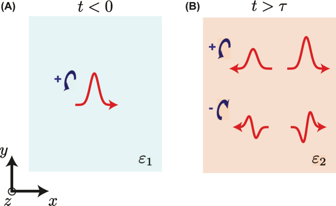
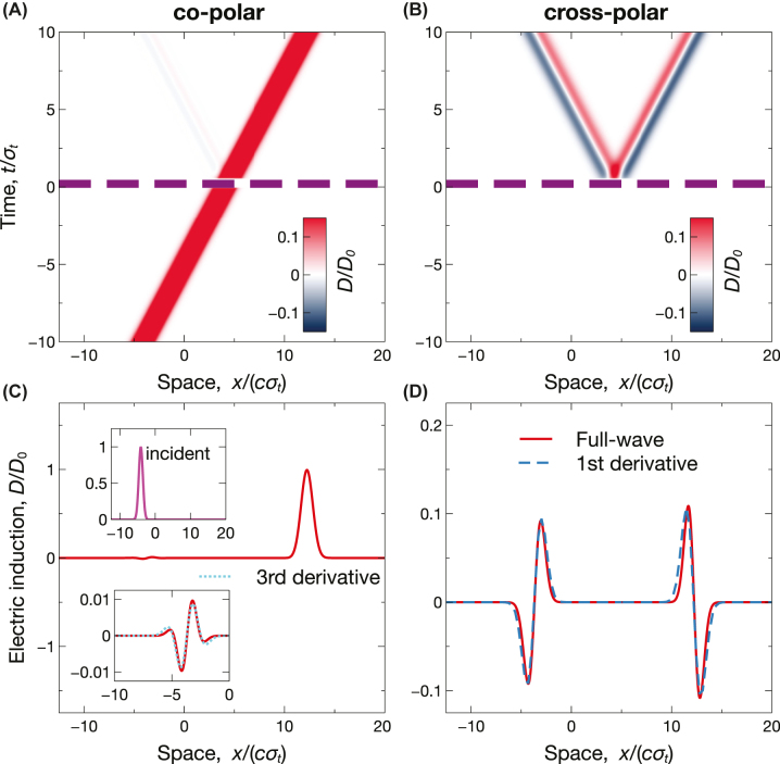
Temporal metamaterials, based on time-varying constitutive properties, offer new exciting possibilities for advanced field manipulations. In this study, we explore the capabilities of anisotropic temporal slabs, which rely on abrupt changes in time from isotropic to anisotropic response (and vice versa). Our findings show that these platforms can effectively manipulate the wave-spin dimension, allowing for a range of intriguing spin-controlled photonic operations. We demonstrate these capabilities through examples of spin-dependent analog computing and spin-orbit interaction effects for vortex generation. These results provide new insights into the field of temporal metamaterials, and suggest potential applications in communications, optical processing and quantum technologies.

Keywords: analog computing; anisotropy; metamaterials; spin-orbit interaction; time-varying.

Figure 1:

Schematic representation of an anisotropic temporal slab (details in the text).

Figure 2:

Schematic illustration of spin-dependent analog computing. (A) A wavepacket with a positive spin (i.e., LHC) impinges in the initial medium. (B) After the short-pulsed anisotropic temporal modulation (t > τ), the co-polarized reflected (backward) and transmitted (forward) wavepacket exhibit the same profile as the impinging one, whereas the cross-polarized ones are proportional to its first derivative.

Figure 3:

Example of spin-dependent analog computing. Anisotropic short-pulsed temporal slab with ɛ _⊥ = 1, ɛ _‖ = 3, ɛ ₁ = 1, ɛ ₂ = 4, and τ = 0.5σ _t , excited by the incident Gaussian wavepacket in Equation (9) [see inset in panel (C)]. (A), (B) Space-time maps [normalized electric induction, computed from Equations (8)], for co-polar and cross-polar responses, respectively. The thick purple-dashed lines indicate the temporal boundaries. (C), (D) Corresponding spatial cuts at t = 10σ _t , computed via full-wave simulations. The superposed blue-dashed curves indicate the expected first derivatives.

Figure 4:

Example of spin-dependent analog computing. Anisotropic short-pulsed temporal slab with ɛ _⊥ = 1, ɛ _‖ = 3, ɛ ₁ = ɛ ₂ = 1, and τ = 0.5σ _t , excited by the incident Gaussian wavepacket in Equation (9) [see upper inset in panel (C)]. (A), (B) Space-time maps [normalized electric induction, computed from Equations (8)], for co-polar and cross-polar responses, respectively. The thick purple-dashed lines indicate the temporal boundaries. (C), (D) Corresponding spatial cuts at t = 10σ _t , computed via full-wave simulations. The superposed blue-dashed curves indicate the expected first derivatives. The lower inset in panel (C) shows a magnified view of the reflection (backward) response.

Figure 5:

Example of spin-dependent analog computing. Anisotropic short-pulsed temporal slab with ɛ _⊥ = 1, ɛ _‖ = 3, ɛ ₁ = ɛ ₂ = 1.5, and τ = 0.5σ _t , excited by the incident Gaussian wavepacket in Equation (9) [see upper inset in panel (C)]. (A), (B) Space-time maps [normalized electric induction, computed from Equations (8)], for co-polar and cross-polar responses, respectively. The thick purple-dashed lines indicate the temporal boundaries, and the color scale in panel (A) is suitably saturated so as to show the weakest waveform. (C), (D) Corresponding spatial cuts at t = 10σ _t , computed via full-wave simulations. The superposed blue-dashed and cyan-dotted curves indicate the expected first and third derivatives, respectively. The lower inset in panel (C) shows a magnified view of the reflection (backward) response.

Figure 6:

Example of spin-dependent analog computing. (A) Two anisotropic short-pulsed temporal slabs with ɛ _⊥ = 1, ɛ _‖ = 3, ɛ ₁ = ɛ ₂ = 1.5, and τ = 0.5σ _t , starting at t = 0 and t = 10σ _t , excited by the incident Gaussian wavepacket in Equation (9). (B), (C) Spatial cuts of normalized electric induction at t = 40σ _t , computed via full-wave simulations, for co-polar and cross-polar responses, respectively. The insets show some magnified views of the responses. The superposed blue-dashed and green-dotted curves indicate the expected first and second derivatives, respectively.

Figure 7:

Schematic illustration of the spin–orbit interactions and vortex generation. (A) A circularly polarized Bessel-type beam with positive spin (i.e., LHC) and no topological charge (ℓ = 0) impinges in the initial medium. (B) After the anisotropic temporal modulation (t > τ), the beam is generally converted into cross-polarized reflected (backward) and transmitted (forward) vortex beams with topological charge ℓ = 2. If the initial and final permittivities are different (ɛ ₁ ≠ ɛ ₂), frequency conversion (from ω ₁ to ω ₂) is attained too. Note the different incidence conditions by comparison with the scenario in Figure 2.

Figure 8:

Example of spin–orbit interaction effects (vortex generation). Anisotropic temporal slab with ɛ _⊥ = 8, ɛ _‖ = 1.946, ɛ ₁ = ɛ ₂ = 1 and $\tau =3\sqrt{2}T$ , excited by a time-harmonic Bessel-type beam as in Equations (10), with period T, wavelength λ = cT, and characteristic wavenumbers k ₀ = 2π/λ and k _0⊥ = π/λ. (A), (B) Transverse wavefronts (normalized electric induction) of impinging and transmitted (forward) cross-polarized beams, respectively, computed via full-wave simulations at t = −T and t = 19.75T, respectively. All other (co- and cross-polarized) scattering terms are below $\sim 10^{-7}$ in the normalized scale.

References

1. Engheta N. Metamaterials with high degrees of freedom: space, time, and more. Nanophotonics. 2021;10(1):639–642. doi: 10.1515/nanoph-2020-0414. - DOI
1. Caloz C., Deck-Léger Z. Spacetime metamaterials—part I: general concepts. IEEE Trans. Antenn. Propag. 2020;68(3):1569–1582. doi: 10.1109/tap.2019.2944225. - DOI
1. Caloz C., Deck-Léger Z. Spacetime metamaterials—part II: theory and applications. IEEE Trans. Antenn. Propag. 2020;68(3):1583–1598. doi: 10.1109/tap.2019.2944216. - DOI
1. Morgenthaler F. R. Velocity modulation of electromagnetic waves. IRE Trans. Microw. Theor. Tech. 1958;6(2):167–172. doi: 10.1109/tmtt.1958.1124533. - DOI
1. Oliner A. A., Hessel A. Wave propagation in a medium with a progressive sinusoidal disturbance. IRE Trans. Microw. Theor. Tech. 1961;9(4):337–343. doi: 10.1109/tmtt.1961.1125340. - DOI
LinkOut - more resources