A tutorial on pharmacometric Markov models

Abstract

The Markov chain is a stochastic process in which the future value of a variable is conditionally independent of the past, given its present value. Data with Markovian features are characterized by: frequent observations relative to the expected changes in values, many consecutive same-category or similar-value observations at the individual level, and a positive correlation observed between the current and previous values for that variable. In drug development and clinical settings, the data available commonly present Markovian features and are increasingly often modeled using Markov elements or dedicated Markov models. This tutorial presents the main characteristics, evaluations, and applications of various Markov modeling approaches including the discrete-time Markov models (DTMM), continuous-time Markov models (CTMM), hidden Markov models, and item-response theory model with Markov sub-models. The tutorial has a specific emphasis on the use of DTMM and CTMM for modeling ordered-categorical data with Markovian features. Although the main body of this tutorial is written in a software-neutral manner, annotated NONMEM code for all key Markov models is included in the Supplementary Information.

FIGURE 1

Recommended visualizations to explore the Markovian feature of the observed data of an ordered‐categorical variable. As an example, an ordered‐categorical variable is used: It considers the three ordered categories of (i) no response, (ii) partial response, and (iii) full response for a typical subject receiving placebo. The longitudinal profile of the ordered‐categorical variable values is shown stratified by data without (Panel a) and with Markovian features (Panel b). Correlation plots of current versus previous response categories are also shown, stratified by data without (Panel c) and with Markovian feature (Panel d). For panels c and d: The time lapse between the current and previous observation is not accounted for; the size of the dots corresponds to the number of counts for the specific category; the thick solid line represents a generalized additive mode smoothing of the data. The n represents the count for unique transition categories.

FIGURE 2

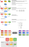
Schematic representation of different Markov models: A proportional odds model with Markov element(s) (i.e., not a Markov model, Panel a); a discrete‐time Markov model (DTMM) (Panel b); a continuous‐time Markov model (CTMM) with default parameterization and equilibrium time (ET) parameterization that underpins the minimal continuous‐time Markov model (mCTMM) (Panel c); an item‐response theory (IRT) model with Markov sub‐models joined by common underlying individual latent variable $D_i$ (Panel d); and a hidden Markov model (Panel e). These models are exemplified for a variable, sub‐variable, or hidden Markov element with three ordered categories (named 1, 2, and 3). The DTMM and CTMM account for dropout using an absorbing state. Estimated or fixed parameters are written in black and derived parameters are written in gray. The schematic is inspired by Figure 1 in the paper published by Schindler and Karlsson.

FIGURE 3

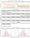
Recommended visual predictive checks to evaluate model fit of data with Markovian features for an ordered‐categorical variable. As an example, an ordered‐categorical variable is used: It considers the three ordered categories of (i) no response, (ii) partial response, and (iii) full response for 50 subjects receiving placebo or 100 mg of a hypothetical drug. Visual predictive check for the longitudinal proportion of subjects in different categories of the ordered‐categorical variable, colored by category and stratified by treatment group (Panel a). Visual predictive check for the longitudinal proportion of subjects in different unique transition categories, stratified by transition category and treatment group (Panel b). Visual predictive check to evaluate the model's ability to describe a metric of interest, mean number of days with full response in this example (Panel c). In both Panel a and b, the thick solid lines correspond to the observed proportion of subjects and the shaded areas correspond to the 95% confidence interval of the simulated proportions. In Panel c, the thick blue vertical lines represent the observed metric of interest; the histograms show the distribution of the simulated metric of interest; and the dashed vertical red lines correspond to the 95% confidence interval of the simulated metric of interest.

FIGURE 4

Continuous‐time Markov model (CTMM) application example. Longitudinal probability of a typical subject predicted by the CTMM without reset of probabilities at time of observations, colored by category of an ordered categorical variable, and stratified by treatment arm. As an example, an ordered‐categorical variable is used: It considers the three ordered categories of (i) no response, (ii) partial response, and (iii) full response, with the possibility to dropout from each category, for 50 subjects receiving placebo or 100 mg of a hypothetical drug.

FIGURE 5

Conceptual illustration of probability changing over time as described by a continuous‐time Markov model for a typical subject, stratified by ordered categories and dropout. As an example, an ordered‐categorical variable is used: It considers the three ordered categories (named 1, 2, and 3) of (i) no response, (ii) partial response, and (iii) full response, with the possibility to dropout from each category, for a typical subject receiving 100 mg of a hypothetical drug.

FIGURE 6

Decision tree for choosing the type of Markov model suitable to describe observed data with Markovian features.

References

1. Silber HE, Kjellsson MC, Karlsson MO. The impact of misspecification of residual error or correlation structure on the type I error rate for covariate inclusion. J Pharmacokinet Pharmacodyn. 2009;36(1):81‐99. - PubMed
1. Karlsson MO, Beal SL, Sheiner LB. Three new residual error models for population PK/PD analyses. J Pharmacokinet Biopharm. 1995;23(6):651‐672. - PubMed
1. Giltinan MD, David M. Nonlinear Models for Repeated Measurement Data. Routledge; 2017. 360 p.
1. Deng C, Plan EL, Karlsson MO. Approaches for modeling within subject variability in pharmacometric count data analysis: dynamic inter‐occasion variability and stochastic differential equations. J Pharmacokinet Pharmacodyn. 2016;43(3):305‐314. - PubMed
1. Tornøe CW, Overgaard RV, Agersø H, Nielsen HA, Madsen H, Jonsson EN. Stochastic differential equations in NONMEM: implementation, application, and comparison with ordinary differential equations. Pharm Res. 2005;22(8):1247‐1258. - PubMed
LinkOut - more resources