Image analysis techniques for in vivo quantification of cerebrospinal fluid flow

Abstract

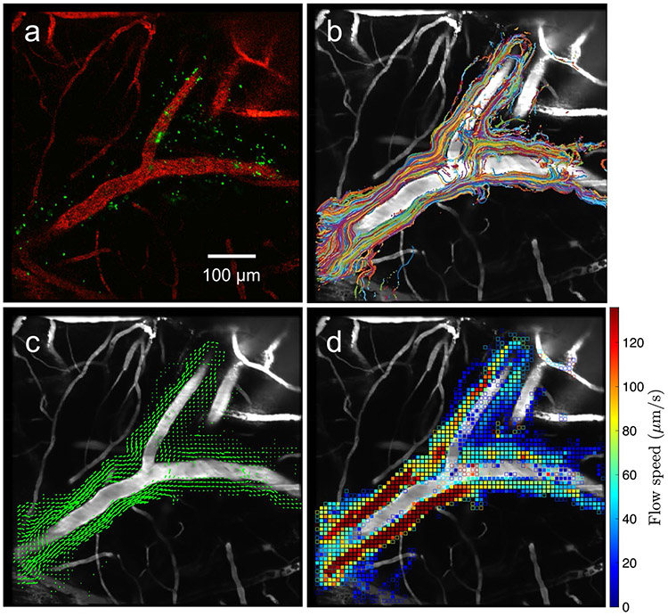
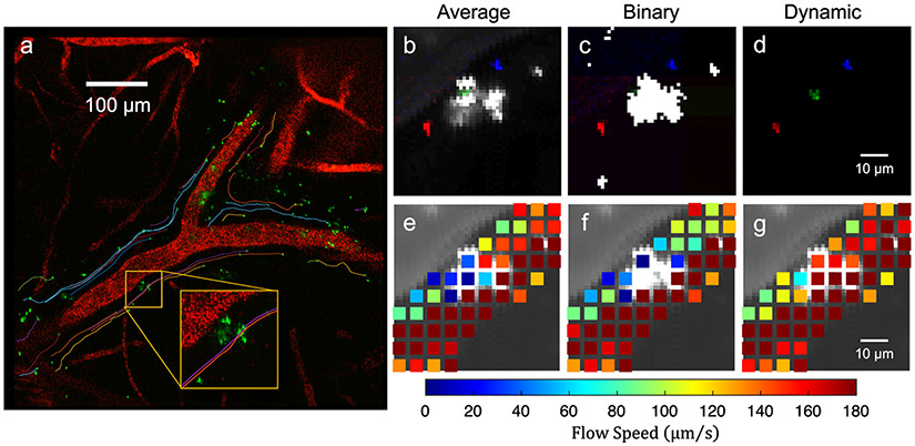
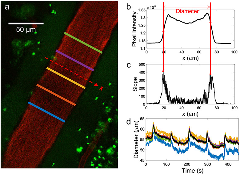
Over the past decade, there has been a tremendously increased interest in understanding the neurophysiology of cerebrospinal fluid (CSF) flow, which plays a crucial role in clearing metabolic waste from the brain. This growing interest was largely initiated by two significant discoveries: the glymphatic system (a pathway for solute exchange between interstitial fluid deep within the brain and the CSF surrounding the brain) and meningeal lymphatic vessels (lymphatic vessels in the layer of tissue surrounding the brain that drains CSF). These two CSF systems work in unison, and their disruption has been implicated in several neurological disorders including Alzheimer's disease, stroke, and traumatic brain injury. Here, we present experimental techniques for in vivo quantification of CSF flow via direct imaging of fluorescent microspheres injected into the CSF. We discuss detailed image processing methods, including registration and masking of stagnant particles, to improve the quality of measurements. We provide guidance for quantifying CSF flow through particle tracking and offer tips for optimizing the process. Additionally, we describe techniques for measuring changes in arterial diameter, which is an hypothesized CSF pumping mechanism. Finally, we outline how these same techniques can be applied to cervical lymphatic vessels, which collect fluid downstream from meningeal lymphatic vessels. We anticipate that these fluid mechanical techniques will prove valuable for future quantitative studies aimed at understanding mechanisms of CSF transport and disruption, as well as for other complex biophysical systems.

Fig. 1

An example of image analysis to quantify CSF flow through PVSs at the surface of a mouse brain. Fluorescent tracers are injected into the blood (bovine serum albumin) and CSF (1 μm polystyrene microspheres) and then recorded in vivo using two-photon microscopy by imaging through a cranial window. a A snapshot of a pial artery (red) and fluorescent microspheres (green) acquired at 30 Hz. b Superimposed trajectories of the microspheres obtained from PTV, which can be used to visualize the size of the PVSs. c-d Time-averaged (c) 2D velocity field and (d) flow speed (i.e., magnitude of the velocity field) quantifying the net CSF transport

Fig. 2

Example illustrating image registration in the vicinity of a pial artery. a Snapshots from a time series which show a small, gradual translation in the field of view. b Plot of the $x$-directional and $y$-directional translations that occur in time series, computed via cross-correlation with a reference frame; these translations are used for image registration. c–d Comparison of images at $t=0\mathrm{s}$ (green) and $t=950\mathrm{s}$ (magenta) (c) before and (d) after registration is performed

Fig. 3

Comparison of masking methods. a Image of a pial artery with colored curves indicating the tracking of fluorescent microspheres flowing in the adjacent PVSs. No background has been subtracted for this image. (Inset) A zoomed-in image of a region containing a stagnant microsphere aggregate, which may lead to erroneous measurements of zero velocity if not properly masked. b–d Plots characterizing three different masking techniques (average, binary, and dynamic masking), with the mask superimposed in white/gray. Three sequential unmasked images are also superimposed in red, green, and blue indicating the trajectory of a flowing particle. e–g Net flow speed (i.e., the magnitude of the time-averaged velocity) obtained from particle tracking for a long time series with the indicated masking technique applied. e Average masking incompletely masks the region with stuck particles, leading to erroneous low-velocity measurements. f Binary masking completely removes measurements from the portion of the domain with stuck particles. g Dynamic masking leads to the best results with large velocities near the center of the channel, as expected, and no measurement voids, as in f

Fig. 4

Parameter selections for PTV. a Plots with two $y$-axes characterizing the mean length of the particle tracks (blue) and the number of particle tracks (orange) for variations in: (top) threshold (minimum pixel intensity value used to identify particles), (middle) minimum area (minimum number of neighboring pixels above threshold required to identify a particle), and (bottom) maximum displacement (maximum allowable distance between particle’s predicted and actual location when tracking). b–c Visualization of particle area as the pixel intensity threshold changes. Particles are identified more often and more reliably for lower threshold values, as long as the threshold is above the noise floor. d Higher maximum displacement increases the number of tracks, but the length of the tracks is modestly lowered. The mean track length decreases because of erroneous tracking when maximum displacement is excessively large, leading to poor kinematic predictions that result in tracking failures. This erroneous tracking appears as a sudden sharp turn in a particle trajectory and is more prevalent for a maximum displacement of 20 (bottom) than 8 (middle). For the images analyzed here, the resolution is 1.17 μm/pixel at 29.53 Hz. For tests depicted in (a), the variable on the $x$-axis was varied while the other two variables were fixed (threshold 3000, minimum area 3, and maximum displacement 15)

Fig. 5

Quantitative measurements of changes in arterial diameter. a Two-photon microscopy image of a pial artery (red) and its adjacent PVS with several stagnant aggregated particles (green blobs). The solid colored lines indicate measurements of arterial diameter, while the dashed red line indicates an example region over which we interpolate the pixel intensity to identify the vessel diameter. b Plot of the interpolated pixel intensity along the red dashed line in (a). c The second-order accurate central finite difference of the pixel intensity profile in (b). The edges of the vessel are identified based on the two local maxima, indicated by the solid, vertical red lines. d Time series of the change in artery diameter with locations corresponding to the same color scheme used in panel (a). The solid black curve corresponds to the median across space evaluated at each instant of time. Note that the large amplitude oscillations with a period of about 9 s arise due to neurovascular coupling (alterations in local blood flow due to neuronal activity) and not cardiac pulsations

Fig. 6

Image analysis techniques presented above, applied to a cervical lymphatic vessel. a TPM image of a cervical lymphatic vessel visualized using fluorescent dye (green) and microspheres (red). Magenta arrows represent instantaneous velocity of the particles inside the vessel. Three perpendicular colored lines indicate profile locations where the vessel diameter is measured. b A time series of normalized cross-correlation values with a moving average of 60 frames applied for three different cases: unregistered images (gray curve), images registered using rigid translation only (green curve), and images registered using both rigid translation and rotation (purple curve). c A time series of the spatially-averaged instantaneous velocity obtained from particle tracking. Positive value indicates prograde flow, while negative value indicates retrograde flow. d A time series of the instantaneous vessel diameter which reveals large amplitude contractions of the vessel that closely matches the timing of changes in fluid velocity plotted in (c)

References

1. Abbott NJ (2004) Evidence for bulk flow of brain interstitial fluid: significance for physiology and pathology. Neurochem Int 45(4):545–552 - PubMed
1. Abbott NJ, Pizzo ME, Preston JE, Janigro D, Thorne RG (2018) The role of brain barriers in fluid movement in the CNS: is there a ‘glymphatic’ system? Acta Neuropathol 135(3):387–407 - PubMed
1. Agarwal N, Carare RO (2021) Cerebral vessels: an overview of anatomy, physiology, and role in the drainage of fluids and solutes. Front Neurol 11:1748 - PMC - PubMed
1. Ahn JH, Cho H, Kim J-H, Kim SH, Ham J-S, Park I, Suh SH, Hong SP, Song J-H, Hong Y-K, Jeong Y, Park S-H, Koh GY (2019) Meningeal lymphatic vessels at the skull base drain cerebrospinal fluid. Nature 572(7767):62–66. 10.1038/s41586-019-1419-5 - DOI - PubMed
1. Albargothy NJ, Johnston DA, MacGregor-Sharp M, Weller RO, Verma A, Hawkes CA, Carare RO (2018) Convective influx/glymphatic system: tracers injected into the CSF enter and leave the brain along separate periarterial basement membrane pathways. Acta Neuropathol 136(1):139–152 - PMC - PubMed
LinkOut - more resources