DiffMAP-GP: Continuous 2D diffusion maps from particle trajectories without data binning using Gaussian processes

Abstract

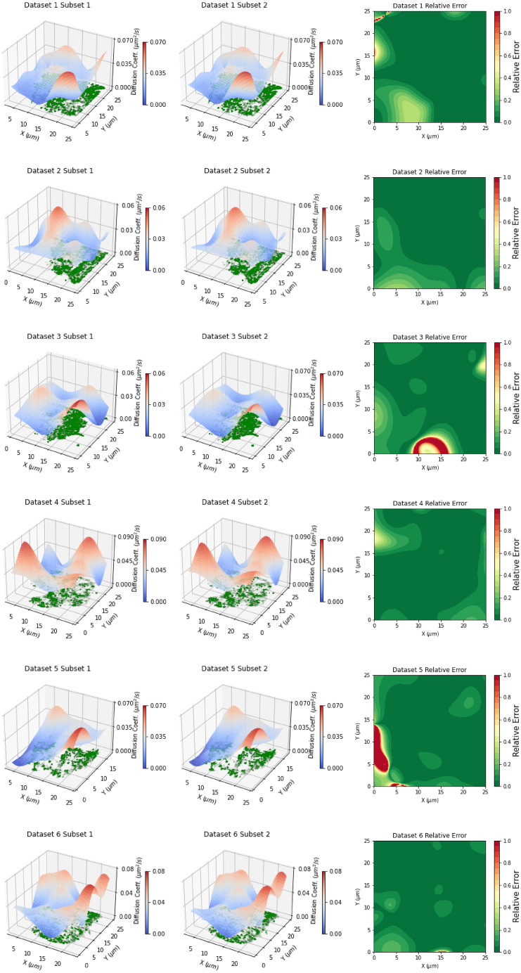
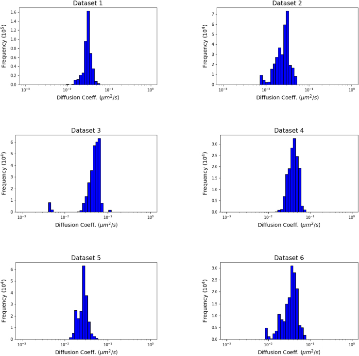
Diffusion coefficients often vary across regions, such as cellular membranes, and quantifying their variation can provide valuable insight into local membrane properties such as composition and stiffness. Toward quantifying diffusion coefficient spatial maps and uncertainties from particle tracks, we develop a Bayesian framework (DiffMAP-GP) by placing Gaussian process (GP) priors on the family of candidate maps. For sake of computational efficiency, we leverage inducing point methods on GPs arising from the mathematical structure of the data giving rise to nonconjugate likelihood-prior pairs. We analyze both synthetic data, where ground truth is known, as well as data drawn from live-cell single-molecule imaging of membrane proteins. The resulting tool provides an unsupervised method to rigorously map diffusion coefficients continuously across membranes without data binning.

Figure 1

Schematic representation of DiffMAP-GP. DiffMAP-GP is a framework using single-particle localizations forming trajectories as input and outputs a continuous mapping of the diffusion coefficient as a function of space without binning or other forms of data downsampling. On the left is a single frame from a fluorescence microscopy frame stack labeled in orange to reflect membrane protein trajectories. These trajectories are the input into our model identifying the spatial diffusion coefficient map (plotted on the right) of the highest probability. Above the arrow is the posterior, a central quantity of DiffMAP-GP, which is the probability over all maps given (conditioned on) the data. The posterior here is maximized over all (technically infinite) candidate maps to generate the diffusion coefficient map plotted on the right. The green dots on the right identify the localizations of membrane proteins (“particles”) used in deducing the diffusion coefficient map. The links between localizations forming tracks, for clarity alone, are not shown.

Figure 2

Learning diffusion coefficient maps from synthetic data. Each row here represents an analysis of a unique synthetic data set. The first column of each row (a, d, and g) shows the true diffusion coefficient map used in synthetic data simulation and the second column (b, e, and h) plots the diffusion coefficient map inferred by the method, with the synthetic data plotted in green below the surface. As can be seen in the second column, we progressively increase the number of localizations, $5\times {10}^3$, ${10}^5$, and $2\times {10}^5$, respectively. The third column (c, f, and i) plots the relative error between the Ground Truth Diffusion Map and the Inferred Diffusion Map as a function of space computed according to Eq. (13).

Figure 3

Learning diffusion coefficient maps from experimental data. Here, we visualize the inferred diffusion coefficient map from six different experimental data sets, each from different cells. The green points at the bottom of each plot represent DC-SIGN wild-type (a–c) and N80A (d–f) ${10}^5$ localizations from trajectories analyzed for each set. The surfaces plotted are the inferred maps from the method and, as we describe in the main text, they exhibit large bumps toward the edge of the field of view where there is little to no data.

Figure 4

Self-consistency check on experimental data. We subsetted each experimental data set into half and ran the algorithm on each half. Each row above represents a unique data set. The first two columns coincide with the inferred map plotted with the respective data half below. The third column is the relative error between the two inferred maps.

Figure 5

Robustness of inference on synthetic data. Here, we evaluate our model’s robustness with respect to varying diffusion maps, including a flat map (a), a single peak (b), and overlapping waves (c and d), and the amount of available data. We have selected a consistent 25 $\mu {\mathrm{m}}^2$ field of view.

Figure 6

Self-consistency by subsetting trajectories. Here, we zoom to the most trajectory-rich region of our first experimental data set. We subset the data in this region by randomly splitting the trajectories into two groups. Then we run our inference scheme on each subset individually (a) and (b). Then we compare by plotting relative error (c).

Figure 7

Histogram of estimated diffusion coefficients. For each of the six experimental data sets considered throughout, we visualize the frequency of estimated diffusion coefficients at all positions of every trajectory. Specifically, we use the inferred diffusion maps shown in Fig. 3 to determine the diffusion values at all protein localizations in the data. This evaluation is done using the interpolation scheme defined in Eq. (9).

Figure 8

Localization density for experimental datasets. The localization density of the six experimental data sets featured in Fig. 3 is shown above via a Gaussian KDE. We notice the data become increasingly sparse toward the edges of the field of view, with some regions containing no data at all.

Figure 9

Mean-square displacements for experimental datasets. Here, we show the mean-square displacement (MSD) associated with the experimental data sets shown in Fig. 3. Specifically, we plot the MSD of all trajectories at least 100 localizations long, equivalent to 3.3 s. For each data set this amounts to the following numbers of trajectories considered: 464 (a), 486 (b), 304 (c), 219 (d), 276 (e), and 169 (f). The average MSD is plotted as a solid line and the shaded blue region represents the smallest interval that contains 95% of the trajectories considered. The average MSD is linear for all data sets, with large variance consistent with large changes in diffusion coefficient seen across the data.

Figure 10

Comparison between binning method versus DiffMAP-GP. Here, we compare our method to a traditional binning method. (a) is the true diffusion surface used to simulate data, (b) is the inferred diffusion map from a binned MLE, (c) is the relative error between the binned MLE and ground truth, (d) is the inferred map using our method, DiffMAP-GP, and (e) is the relative error between our inferred map and the ground truth. In flat regions both methods perform well, staying below 10% relative error. In areas of rapidly changing diffusion, the binned MLE fails entirely, above 90% relative error, while DiffMAP-GP is able to stay below 40%.

References

1. Cheng X., Smith J.C. Biological Membrane Organization and Cellular Signaling. Chem. Rev. 2019;119:5849–5880. - PubMed
1. Casares D., Escribá P.V., Rosselló C.A. Membrane Lipid Composition: Effect on Membrane and Organelle Structure, Function and Compartmentalization and Therapeutic Avenues. Int. J. Mol. Sci. 2019;20:2167. - PMC - PubMed
1. Vereb G., Szöllosi J., et al. Damjanovich S. Dynamic, yet structured: The cell membrane three decades after the Singer-Nicolson model. Proc. Natl. Acad. Sci. USA. 2003;100:8053–8058. - PMC - PubMed
1. Jacobson K., Liu P., Lagerholm B.C. The Lateral Organization and Mobility of Plasma Membrane Components. Cell. 2019;177:806–819. - PMC - PubMed
1. Ohkubo T., Shiina T., et al. Mio K. Visualizing Intramolecular Dynamics of Membrane Proteins. Int. J. Mol. Sci. 2022;23 - PMC - PubMed
Substances
LinkOut - more resources