

Challenges in data-driven geospatial modeling for environmental research and practice
- PMID: 39702456
- PMCID: PMC11659326
- DOI: 10.1038/s41467-024-55240-8
Challenges in data-driven geospatial modeling for environmental research and practice
Abstract
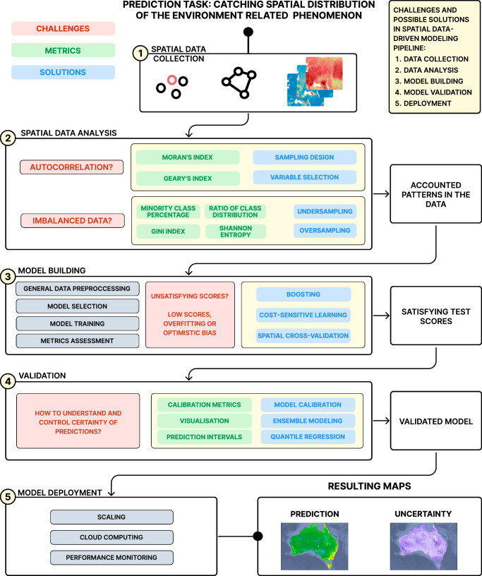
Machine learning-based geospatial applications offer unique opportunities for environmental monitoring due to domains and scales adaptability and computational efficiency. However, the specificity of environmental data introduces biases in straightforward implementations. We identify a streamlined pipeline to enhance model accuracy, addressing issues like imbalanced data, spatial autocorrelation, prediction errors, and the nuances of model generalization and uncertainty estimation. We examine tools and techniques for overcoming these obstacles and provide insights into future geospatial AI developments. A big picture of the field is completed from advances in data processing in general, including the demands of industry-related solutions relevant to outcomes of applied sciences.
© 2024. The Author(s).
Conflict of interest statement
Competing interests: The authors declare no competing interests.
Figures

Similar articles
-
Integrating Multiscale Geospatial Environmental Data into Large Population Health Studies: Challenges and Opportunities.Toxics. 2022 Jul 20;10(7):403. doi: 10.3390/toxics10070403. Toxics. 2022. PMID: 35878308 Free PMC article.
-
Emerging trends in geospatial artificial intelligence (geoAI): potential applications for environmental epidemiology.Environ Health. 2018 Apr 17;17(1):40. doi: 10.1186/s12940-018-0386-x. Environ Health. 2018. PMID: 29665858 Free PMC article.
-
Consensus statements on the current landscape of artificial intelligence applications in endoscopy, addressing roadblocks, and advancing artificial intelligence in gastroenterology.Gastrointest Endosc. 2025 Jan;101(1):2-9.e1. doi: 10.1016/j.gie.2023.12.003. Epub 2024 Apr 17. Gastrointest Endosc. 2025. PMID: 38639679
-
AI-based processing of future prepared foods: Progress and prospects.Food Res Int. 2025 Feb;201:115675. doi: 10.1016/j.foodres.2025.115675. Epub 2025 Jan 4. Food Res Int. 2025. PMID: 39849794 Review.
-
ASAS-NANP symposium: mathematical modeling in animal nutrition: limitations and potential next steps for modeling and modelers in the animal sciences.J Anim Sci. 2022 Jun 1;100(6):skac132. doi: 10.1093/jas/skac132. J Anim Sci. 2022. PMID: 35419602 Free PMC article. Review.
Cited by
-
Identification of flood vulnerability areas using analytical hierarchy process techniques in the Wuseta watershed, Upper Blue Nile Basin, Ethiopia.Sci Rep. 2025 Aug 6;15(1):28680. doi: 10.1038/s41598-025-13822-6. Sci Rep. 2025. PMID: 40770249 Free PMC article.
References
-
- Gewin, V. Mapping opportunities. Nature427, 376–377 (2004). - PubMed
-
- Fick, S. E. & Hijmans, R. J. Worldclim 2: new 1-km spatial resolution climate surfaces for global land areas. Int. J. Climatol.37, 4302–4315 (2017).
-
- Chuvieco, E. et al. Historical background and current developments for mapping burned area from satellite earth observation. Remote Sens. Environ.225, 45–64 (2019).
-
- Reichstein, M. et al. Deep learning and process understanding for data-driven earth system science. Nature566, 195–204 (2019). - PubMed
-
- Brown, C. F. et al. Dynamic world, near real-time global 10 m land use land cover mapping. Sci. Data9, 251 (2022).
Publication types
LinkOut - more resources
Full Text Sources
