The International Bathymetric Chart of the Arctic Ocean Version 5.0

Abstract

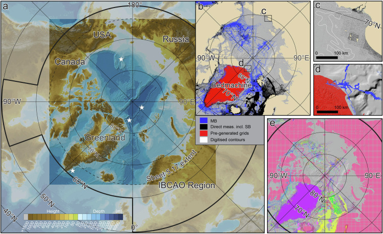
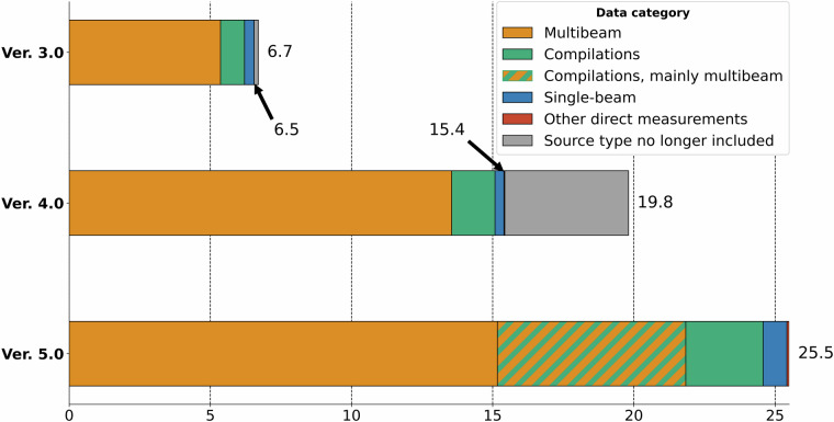
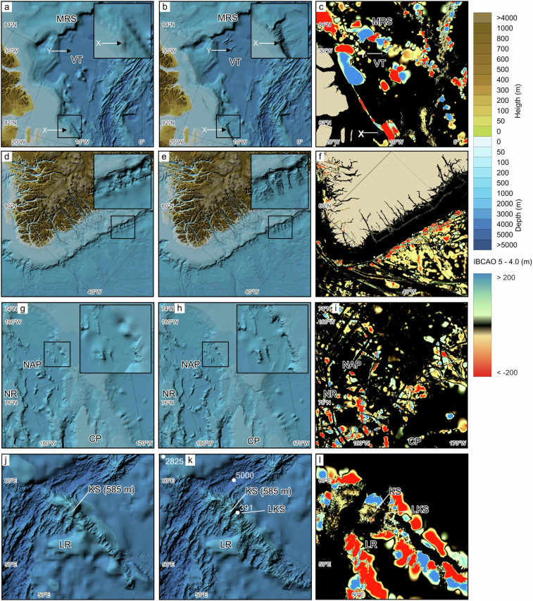
Knowledge about seafloor depth, or bathymetry, is crucial for various marine activities, including scientific research, offshore industry, safety of navigation, and ocean exploration. Mapping the central Arctic Ocean is challenging due to the presence of perennial sea ice, which limits data collection to icebreakers, submarines, and drifting ice stations. The International Bathymetric Chart of the Arctic Ocean (IBCAO) was initiated in 1997 with the goal of updating the Arctic Ocean bathymetric portrayal. The project team has since released four versions, each improving resolution and accuracy. Here, we present IBCAO Version 5.0, which offers a resolution four times as high as Version 4.0, with 100 × 100 m grid cells compared to 200 × 200 m. Over 25% of the Arctic Ocean is now mapped with individual depth soundings, based on a criterion that considers water depth. Version 5.0 also represents significant advancements in data compilation and computing techniques. Despite these improvements, challenges such as sea-ice cover and political dynamics still hinder comprehensive mapping.

Fig. 1

Overview maps illustrating Arctic Ocean bathymetry and source data for the compilation of IBCAO 5.0. (a) Bathymetry based on IBCAO 5.0. Two versions are available: one with under-ice topography of Greenland (shown), and another with the ice-sheet surface topography, both based on BedMachine Version 5 DMT. The bold black line shows the Seabed 2030 Arctic region, for which a geographic DTM is produced and contributed to the global GEBCO DTM. The square region shown in brighter colours represents the more limited extent of the IBCAO DTM. White stars show the locations of detailed comparison between IBCAO 5.0 and 4.0 in Fig. 9. (b) Source data displayed based on the mapping method (MB = Multibeam; SB = Singlebeam). (c) Close-up of the East Siberian Sea depicting soundings from charts (in black) and digitised contours (in white). The nodes of the digitised contours, utilised in the gridding process, may be challenging to discern due to their sparse density. To enhance visibility, several contours are presented as polygons in white. (d) Close-up of North Greenland showing a part of the least mapped area of the Arctic Ocean. (e) Source data displayed as individual data sets using different colours. Note that the high resolution of the IBCAO 5.0 gridded products precludes displaying fine details in overview figures. For detailed information, readers are referred to the downloadable grids.

Fig. 2

Comparison between the three main source data categories in IBCAO 3.0, 4.0 and 5.0. Note that the grey sections of the bars for IBCAO 3.0 and 4.0 represent source data types we no longer count when calculating mapping coverage. See Table 2 for definition of the data categories. A large segment of the “compilations” data category is likely composed of multibeam measurements, although only a rough estimation is currently available.

Fig. 3

Flow chart of the major steps involved in compiling the IBCAO 5.0 grid. The orange headings correspond to sections within Methods describing the main compilation procedures. AWS: Amazon Web Services; TID: Type Identification; SID: Source Identification.

Fig. 4

The gridding procedure shown schematically with all included main steps described in the text. Lightly shaded boxes represent tabular calculations using Pandas, dark shaded boxes represent raster calculations using NumPy whereas intermediate-shaded boxes represent interpolation using PyGMT. Note that this procedure is implemented for the “crude”, “draft” and “final” gridding as shown in Fig. 3.

Fig. 5

Visualisations of the outcome of some of the main gridding steps. The island is Kvitøya in eastern Svalbard. (a) Block median at 2,000 × 2,000 m of all data including both low- and high-resolution data after calculation step 5. (b) Blockmedian at 100 × 100 m after upsampling, showing the result of calculation step 5. (c) Low resolution 2,000 × 2,000 m interpolated, smoothed and resampled base grid produced using the blockmedian grid and the Generic Mapping Tools (GMT) spline in tension function in step 8. (d) Difference between (b,c), after applying a 20 grid cell empty buffer zone around high-resolution data in calculation step 10. (e) Interpolated difference values filling the buffer zones to make a smooth transition between high- and low-resolution data, also in step 10. (f) Restored final grid where the grid in e is added to b.

Fig. 6

Illustration of how a substantially faster incremental gridding is frequently employed to ingest new data, while full gridding of the entire DTM regions is typically reserved for occasions when new DTM versions are published or significant edge effects are observed around included datasets.

Fig. 7

Examples of new major depth sources in IBCAO 5.0. (a) Soundings digitised from 150 published Russian navigational charts. (b) Close-up showing the sounding density around Russian Severnaya Zemlya. (c) Depths from seafloor groundings of Argo Floats.

Fig. 8

Comparison between different versions of IBCAO by subtracting one grid from the other. Black to dark colours show no or minor changes. (a) IBCAO 5.0 - 4.0. (b) IBCAO 4.0 - 3.0.

Fig. 9

Comparison between IBCAO 4.0 and 5.0 in four selected areas. Locations of the areas are indicated in Fig. 1. The left column depicts IBCAO 4.0, the middle column shows IBCAO 5.0, and the right column displays the depth difference between the two (IBCAO 5.0 - 4.0). Colours toward blue indicate that IBCAO 5 is shallower than IBCAO 4.0, whereas colours towards red show the opposite. (a–c) Area north of the North Greenland continental margin and adjacent deep waters. X marks the significant change from IBCAO 4.0 to 5.0 in the portrayal and location of the continental shelf break and slope. Y shows where new multibeam bathymetry reveals a texture of the Voronov Terrace (VT). MRS = Morris Jesup Spur. (d–f) Southeast Greenland continental slope where new multibeam data reveal a typical slope morphology dominated by canyons. (g–i) Section of the Chukchi Borderland comprising the Northwind Ridge (NR), Northwind Abyssal Plain (NAP) and Chukchi Plateau (CP). Here several new multibeam tracks reveal steeper slopes surrounding the NAP. (j–l) The Langeth Ridge (LR) forming a part of the extensive Gakkel Ridge; the only active spreading ridge in the Arctic Ocean, which has the World ocean’s slowest spreading rates varying between about 6 and 13 mm/year.

Fig. 10

3D view of the Langseth Ridge area shown in Fig. 9j-l. The visualisation illustrates an example of when our gridding algorithm works exceptionally well in generating smooth seams between high- and low-resolution source data.

Fig. 11

Examples of issues encountered in IBCAO 5.0. (a) Area west of Svalbard with examples of refractions and wobbly outer beams most likely due to poor sound velocity control during data acquisition. (b) An example east of southern Greenland where the gridding algorithm failed to optimally merge the multibeam bathymetry with the surrounding grid based on sparse source data. (c) An example of digitised depth contours poorly matching multibeam bathymetry.

References

1. Wölfl, A.-C. et al. Seafloor mapping - The challenge of a truly global ocean bathymetry. Front. Mar. Sci. 6, (2019).
1. Edwards, M. H. & Coakley, B. J. SCICEX Investigations of the Arctic Ocean System. Chem. Erde63, 281–328 (2003).
1. Hunkins, K. & Tiemann, W. Geophysical Data Summary for Fletcher’s Ice Island (T3), May 1962-October 1974. 1–219 (1977).
1. Kristoffersen, Y. US ice drift station FRAM-IV: Report on the Norwegian field program. Nor. Polarinst. Rapp.11, 2–60 (1982).
1. Kristoffersen, Y. & Hall, J. K. Hovercraft as a Mobile Science Platform Over Sea Ice in the Arctic Ocean. Oceanography27, 170–179 (2014).