Fourier analysis of signal dependent noise images

Abstract

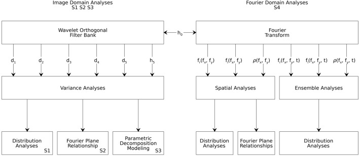
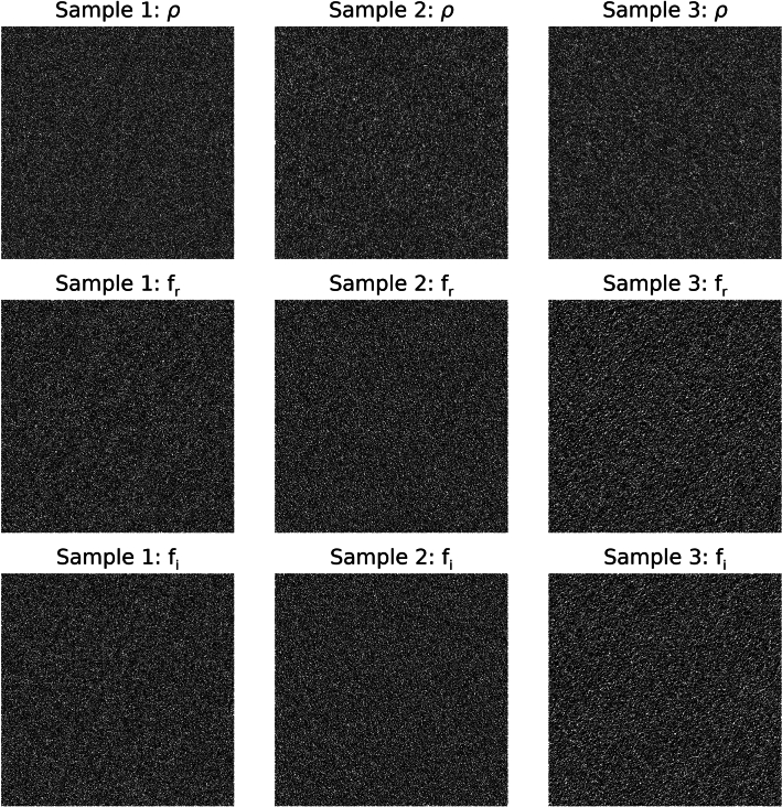
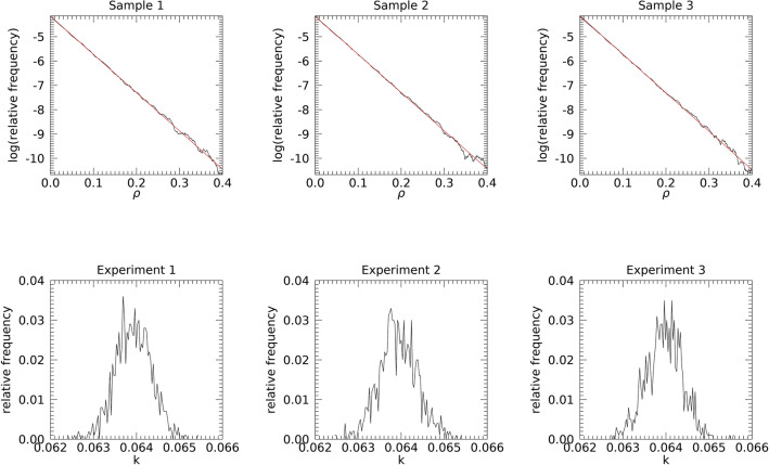
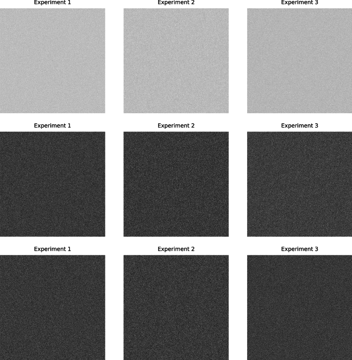
An archetype signal dependent noise (SDN) model is a component used in analyzing images or signals acquired from different technologies. This model-component may share properties with stationary normal white noise (WN). Measurements from WN images were used as standards for making comparisons with SDN in both the image domain (ID) and Fourier domain (FD). The ID wavelet expansion was applied to WN images (n = 1000). Orthogonality conditions were used to parametrically model the variance decomposition, as described in both domains. FD components were investigated with probability density function modeling and summarized measures. SDN images were constructed by multiplying both simulated and clinical mammograms (both with n = 1000) by WN. The variance decomposition for both WN and SDN decreases exponentially as a parametric function of the ID expansion level; expansion image variances for both types of noise were captured similarly in the Fourier plane corresponding with the ID parametric model. The Fourier transform of WN has a uniform power spectrum distributed exponentially; SDN has similar attributes. Fourier inversion of the lag-autocorrelation performed in the FD produced a statistical estimation of the SDN's image factor. These findings are counterintuitive as SDN can be nonstationary in the ID but have stationary attributes in the FD.

Keywords: Fourier analysis; Mammographic simulations; Mammography; Signal dependent noise; Wavelet expansion.

Fig. 1

Investigation flow chart: this shows the overall planned investigation. The four strategies (S1, S2, S3, and S4) have been identified as well. On the left-side, h₀ is analyzed with the wavelet transform (forward and disaggregated inverse); this is equivalent to an input into an orthogonal filter-bank that outputs 6 orthogonal filtered images (d₁–d₅, and h₅) whose sum produces h₀. On the right side, the Fourier transform was taken of each image producing its real and imaginary components and power spectrum [i.e., f_r(f_x, f_y), f_i(f_x, f_y), and ρ(f_x, f_y), respectively, referred to as the Fourier constituents]. When considering all images from a given experiment as an ensemble, the index t was introduced to the respective Fourier coordinates to account for the realization ordering.

Fig. 2

Mammogram region of interest illustration: this shows a mammogram selected at random with the centrally located 500 × 500 pixel region of interest determined with an automated algorithm.

Fig. 3

Fourier plane spectral density bandwidth regions for the expansion images: the left pane shows the spectral cutoffs for a J = 3 wavelet expansion. The right pane shows the same regions further subdivided, where each d_j is expanded into its horizontal, vertical, and diagonal components. The DC component is in the center of the plane.

Fig. 4

Wavelet expansion of sample 1: the 6 expansion images (d₁–d₅ and h₅) for h₀ (white noise)  are shown for a J = 5 decomposition. The texture changes from grainy to lumpy as j increases, and their sum reproduces h₀.

Fig. 5

Wavelet expansion of sample 2: the 6 expansion images (d₁–d₅ and h₅) are shown for h₀ that is a (synthetic mammogram) × noise for a J = 5 expansion. Similarly, the texture changes from grainy to lumpy as j increases, and their sum reproduces h₀.

Fig. 6

Wavelet expansion of sample 3: the 6 expansion images (d₁–d₅ and h₅) are shown for h₀ that is a mammogram × noise for a J = 5 expansion, where h₀ is the region outlined in Fig. 2. Similarly, the texture changes from grainy to lumpy as j increases, and their sum reproduces h₀.

Fig. 7

Fourier plane spatial distributions for the d₁ power spectra for each sample: these show the Fourier plane for a J = 1 expansion for the samples (same Fourier coordinate system and layout Fig. 3). Each row shows the Fourier plane for a given sample. Each pane was contrasted for viewing purposes keeping the level and range the same across all panes. The total region corresponding to d₁ is shown in the first column for each sample. The d₁ images were then expanded into three components: d_1h in the 2nd column; d_1v in the 3rd column; and d_1d in the 4th column for each sample.

Fig. 8

Parametric variance decomposition modeling for the wavelet expansion images: the top row used the respective variance distribution means from each experiment from Table 1. The logarithm of the expansion image standard deviation (σ_j) is plotted (points) as a function of the expansion image index j (i.e., d_j). Each experiment was modeled with the linear relationship (solid line) expressed in Eq. (16) with M_i for the slope and B_i for the intercept. Model parameters for the top row are provided with standard errors parenthetically: Experiment 1, E[M₁] ≈ − 1.02 (0.0) and E[B₁] ≈ 7.79 (0.01); Experiment 2, E[M₂] ≈ − 1.01 (0.0) and E[B₂] ≈ 7.79 (0.01); and Experiment 3, E[M₃] ≈ − 1.02 (0.00) and E[B₃] ≈ 7.79 (0.01). The bottom row shows the analogous plots in the same format for the point estimates derived from the samples: Sample 1, M₁ ≈ − 1.02 (0.00) and B₁ ≈ 7.79 (0.01); Sample 2, M₂ ≈ − 1.01 (0.0) and B₂ ≈ 7.79 (0.01); and Sample 3, M₃ ≈ − 1.00 (0.0) and B₃ ≈ 7.76 (0.03). In all plots, R ≈ − 1.0.

Fig. 9

Fourier domain constituent sample images: top row shows the power spectra (ρ) for the samples selected from each experiment; the middle row shows the respective real parts (f_r) of the Fourier transform (FT) for the samples; and the bottom row shows the respective imaginary parts (f_i) of the FT for the samples. The same window level and range were used in all panes. The Fourier coordinate system is the same as that in Fig. 2. These are well approximated as statistically uniform (flat) chatter with intra row-wise comparisons.

Fig. 10

Fourier domain constituent empirical probability density function samples: the top row shows the power spectra empirical probability density function (pdf) approximations, [g₁(ρ), g₂(ρ), g₁(ρ)], for the three samples shown in Fig. 9. The middle row shows the respective empirical pdfs for the real parts (f_r) of their Fourier transforms (FTs) and the bottom row shows the respective pdfs for their imaginary parts (f_i) of their FTs.

Fig. 11

Power spectra probability density function modeling: the top plots show the natural logarithm of the probability density function (pdfs) from the power spectra (black) modeled as an exponential function and analyzed with linear regression analysis (red) for the samples from each experiment (top row, Fig. 10). The negative inverse of each slope gave: k₁ ≈ 0.063, k₂ ≈ 0.063, and k₃ ≈ 0.064. The standard error (SE) ≈ 0.01 for each k_i, and R ≈ − 1.0 for each plot. The bottom row shows the pdfs top for k_i derived from the 1000 samples from each experiment with distribution means: E[k₁] ≈ 0.063; E[k₂] ≈ 0.063; and E[k₃] ≈ 0.063 with E[R] ≈ − 1.0. SEs were parasitic for each distribution mean. Summaries from the empirical k-distributions (bottom row) and correlation distribution reinforce the findings from the samples (top row).

Fig. 12

Fourier domain mean ensemble images: top row shows the ensemble mean power spectra images, ρ(avg), for each experiment. The real component mean-ensemble images, f_r(avg), are shown in the middle row and the corresponding imaginary component mean-ensemble images, f_i(avg), in the bottom row. Intra row wise comparisons appear similar as uniform chatter.

Fig. 13

Fourier domain ensemble images of the variance for each experiment: top row shows the real component variance-ensemble images, f_r(var), for each experiment, and the second row shows the corresponding imaginary component, variance-ensemble images, f_i(var). Intra row wise comparisons appear similar and uniform.

Fig. 14

Ensemble Fourier domain empirical probability density function (pdf) comparisons for each experiment: in these plots, black, red, and blue curves correspond to experiments 1, 2, and 3 respectively. Each pane has the three curves derived from each experiment over-plotted. In the top row, the left pane shows the pdfs from f_r(avg), the middle pane shows pdfs from f_i(avg), and the right pane shows pdfs from ρ(avg). The second row shows pdfs from f_r(var) in the left pane and pdfs from f_i(var) in the right pane. Within each pane, the curves by observation show agreement.

Fig. 15

Inverse Fourier transform of the power spectrum for each sample: the inverse Fourier transform of the power spectrum for each sample produced a delta function in the image domain. This is an indication that the power spectra were all statistically uniform.

Fig. 16

Fourier domain lag-autocorrelation function for each sample: the top row shows a line through the diagonal of the 2D lag-autocorrelation function (magnitude) of the Fourier transform for each sample. Sample 1 resulted in a delta function, whereas the other samples showed short range lag-correlation. The bottom row shows the square root magnitude of the inverse FT of the Fourier domain lag-autocorrelation function for each sample. Sample 1 is a uniform random noise image as expected, whereas samples 2 and 3 show close resemblance to their respective g(x, y) and m(x, y) images [see Figs. 5 and 6, respectively] as predicted by the work in the Appendix.

References

1. Foi, A., Katkovnik, V., & Egiazarian, E. Signal-dependent noise removal in pointwise shape-adaptive DCT domain with locally adaptive variance. In 2007 15th European Signal Processing Conference, IEEE, pp. 2159–2163 (2007).
1. Torricelli, G., Argenti, F., & Alparone, L. Modelling and assessment of signal-dependent noise for image de-noising. In 2002 11th European signal processing conference, IEEE, pp. 1–4 (2002).
1. Hirakawa, K. Fourier and filterbank analyses of signal-dependent noise. In 2008 IEEE International Conference on Acoustics, Speech and Signal Processing, IEEE, pp. 3517–3520 (2008).
1. Thai, T. H., Retraint, F. & Cogranne, R. Generalized signal-dependent noise model and parameter estimation for natural images. Signal Process.114, 164–170 (2015).
1. Oh, B. T., Kuo, C.-C. J., Sun, S., & Lei, S. Film grain noise modeling in advanced video coding. In Visual Communications and Image Processing 2007, vol. 6508: SPIE, pp. 362–373 (2007).
LinkOut - more resources