Advancing Regulatory Genomics With Machine Learning

Abstract

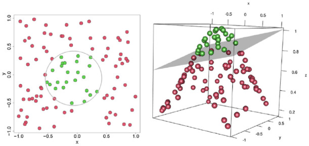
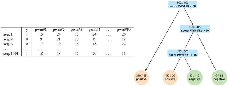
In recent years, several machine learning (ML) approaches have been proposed to predict gene expression signal and chromatin features from the DNA sequence alone. These models are often used to deduce and, to some extent, assess putative new biological insights about gene regulation, and they have led to very interesting advances in regulatory genomics. This article reviews a selection of these methods, ranging from linear models to random forests, kernel methods, and more advanced deep learning models. Specifically, we detail the different techniques and strategies that can be used to extract new gene-regulation hypotheses from these models. Furthermore, because these putative insights need to be validated with wet-lab experiments, we emphasize that it is important to have a measure of confidence associated with the extracted hypotheses. We review the procedures that have been proposed to measure this confidence for the different types of ML models, and we discuss the fact that they do not provide the same kind of information.

Keywords: Regulatory genomics; deep learning; gene expression; machine learning; model interpretation; transcription factor binding sites.

Figure 1.

SVMs work in enlarged spaces. A toy example, illustrating the fact that a linear model in an enlarged space (the gray plane in the 3D space on the right) can define non-linear boundaries in the original space (the gray ellipse in the 2D space on the left), thus providing an accurate classifier for the 2 point classes (red vs. green).

Figure 2.

A toy decision tree inspired from the Epigram method. The learning set involves 1000 sequences (500 positive + 500 negative, see left table). Each sequence is described by the score of 50 PWMs. The decision tree learned from these sequences encodes a set of rules that classify a sequence as positive if the score of PWM#5 is > 80, or if the score of PWM#12 and #21 are > 70 and 85, respectively. Numbers at the top of each node provide the repartition of training sequences in the 2 classes.

Figure 3.

Neural networks. (A) An example of feedforward network with 4 layers. The first layer is connected to 9 input values (in black). The last layer involves a single neuron that outputs a value between 0 and 1. The width and color of the lines represent the weights and signs associated with the inputs to each neuron. (B) An extract of a convolutional neural network that scans DNA sequences. The input sequence is encoded as a 1-hot matrix. A filter of length 5 scans the inputs and computes a convolution at each position. The figure shows 2 convolutions done at 2 different positions with the same filter; filter weights that are associated with non-null input values in the convolution operations are overlined in black. A non-linear activation function then filters the convolution results by removing all values below a given threshold. Finally, the results of these operations are pooled by groups of 4, reducing the output of the convolution to only 4 values. In the figure, only 1 filter is represented, although each convolution layer usually involves dozens or hundreds of filters with their own activation and pooling operations. The results of all filters are then combined in the following layers of the network (not represented here).

Figure 4.

Three approaches for the interpretation of CNNs. (A) Explaining model components. The aim is to identify the motif encoded by each filter of the CNN (the figure illustrates the case for the first filter, in green). A set of sequences (e.g., the training sequences) are presented to the CNN and all sub-sequences that pass the activation threshold of the filter are identified (highlighted in green on the figure). The sub-sequences are then extracted and aligned (middle) and used to build a PWM logo (right) representing the motif encoded by the filter. (B) Explaining model predictions. The aim is to estimate the importance of each nucleotide of a target sequence (top left). The output value of the sequence is computed. In the example, the CNN computes a probability of binding, and the output value of the target sequence is P (1|x) = 0.8. For each nucleotide of the target sequence all possible mutations of that nucleotide are simulated in silico and output values are recomputed (the figure illustrates the case of the nucleotide A at position 5). The difference between the output of the original sequence and of all sequences with a different nucleotide at this position measures the importance of that nucleotide. The procedure is repeated at each position to estimate the importance associated with each nucleotide of the target sequence, which is represented by the height of the letters (bottom). Note that some nucleotides may have negative values if the mutations tend to increase the output value. (C) Exploring model behavior on synthetic sequences. Two sets of synthetic sequences are generated, and the output value of the CNN is computed for each sequence. In the example, all sequences embed a TGATT motif. In addition, the sequences in the second set also have an ATTGC motif located 6 nucleotides on the right of the TGATT motif. The difference in output between sequences from the first and second set thus measures the importance of motif ATTGC when used in combination with motif TGATT. Note that the procedure could be repeated by generating additional sets of sequences with different numbers of nucleotides between the 2 motifs, to investigate the importance of the distance between these motifs.

References

1. Haussler D, Krogh A, Mian S, Sjolander K. Protein modeling using hidden Markov models: analysis of globins. Department of Computer and Information Sciences, University of California at Santa Cruz; 1992. Technical Report UCSC-CRL-92-23.
1. Baldi P, Brunak S. Bioinformatics: The Machine Learning Approach. MIT Press; 1998.
1. Schneider TD, Stormo GD, Gold L, Ehrenfeucht A. Information content of binding sites on nucleotide sequences. J Mol Biol. 1986;188:415-431. - PubMed
1. Stormo GD. Consensus patterns in DNA. Meth Enzymol. 1990;183:211-221. - PubMed
1. Bailey TL, Elkan C. Fitting a mixture model by expectation maximization to discover motifs in biopolymers. Proc Int Conf Intell Syst Mol Biol. 1994;2:28-36. - PubMed
LinkOut - more resources