. 2024 Dec 30;25(1):322.
doi: 10.1186/s13059-024-03458-6.

Descart: a method for detecting spatial chromatin accessibility patterns with inter-cellular correlations

Affiliations

Descart: a method for detecting spatial chromatin accessibility patterns with inter-cellular correlations

Xiaoyang Chen et al. Genome Biol. .

Abstract

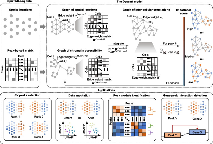
Spatial epigenomic technologies enable simultaneous capture of spatial location and chromatin accessibility of cells within tissue slices. Identifying peaks that display spatial variation and cellular heterogeneity is the key analytic task for characterizing the spatial chromatin accessibility landscape of complex tissues. Here, we propose an efficient and iterative model, Descart, for spatially variable peaks identification based on the graph of inter-cellular correlations. Through the comprehensive benchmarking, we demonstrate the superiority of Descart in revealing cellular heterogeneity and capturing tissue structure. Utilizing the graph of inter-cellular correlations, Descart shows its potential to denoise data, identify peak modules, and detect gene-peak interactions.

Keywords: Data imputation; Feature selection; Gene-peak interactions; Inter-cellular correlations; Peak module; Spatial ATAC-seq; Spatially variable peak.


Conflict of interest statement

Declarations. Ethics approval and consent to participate: Not applicable. Consent for publication: Not applicable. Competing interests: The authors declare that they have no competing interests.

Figures

Fig. 1
Fig. 1
The overview of Descart. Descart first constructs two distinct graphs based on spatial locations of spots and the peak-by-spot matrix, that is, the graph of spatial locations and the graph of chromatin accessibility. Next, Descart integrates the two graphs to derive the graph of inter-cellular correlations and utilizes the self-correlation of each peak within the graph to calculate the importance score. Based on these importance scores, Descart ranks all peaks and selects SV peaks. The SV peaks identified in each iteration are utilized to feedback and update the graph of chromatin accessibility, thereby refining the accuracy of neighborhood relationships among cells. Besides SV peaks identification, Descart can also be applied to data imputation, peak module identification, and detection of gene-peak interaction
Fig. 2
Fig. 2
Benchmarking performance of SV peaks identification on the mouse brain dataset. a Overview for benchmarking results of different methods from three perspectives, that is, the ability to facilitate clustering performance and capture domain-specific signals (see the “Methods” section for further visualization details). b Running time of different methods. c, d Overlapped proportion of SV peaks identified by Descart and baseline methods with domain-specific peaks related to overall domains (c) or each domain (d). Using the “tl.rank_features” function in epiScanpy, we defined the top 100 peaks with the lowest p-values in each domain as domain-specific peaks. e Visualization of domains within the tissue space (left) and the corresponding histological image (right). f Top-ranked SV peak identified by each method on the E13_5-S1 slice, with the raw count values visualized in the tissue space. g Clustering performance using SV peaks identified by Descart and its variants. ATAC-seq-only and spatial-only represents the variants of Descart that only utilizes the graph of chromatin accessibility and the graph of spatial locations, respectively. h, i Clustering performance using SV peaks identified by Descart with a different number of iteration (h), different strategies for peak selection at the initial stage (h), and different multiples of standard distance (i). Clustering performance is evaluated by NMI scores. In b, g, and i, the error bars denote the 95% confidence interval, and the centers of the error bars denote the average value
Fig. 3
Fig. 3
Evaluation for different methods on the mouse embryo dataset and the mixed-species B dataset. a, b Clustering performance evaluated by CHAOS scores using SV peaks identified by different methods on the mouse embryo dataset (a) and the mixed-species B dataset (c), respectively. Due to the lack of well-annotated labels in the two datasets, we are unable to utilize label-dependent metrics for evaluation, such as NMI, ARI, and AMI scores. c, d Running time of different methods on the mouse embryo dataset (b) and the mixed-species B dataset (d), respectively. e, f The histological image (the first plot) and top-ranked SV peak identified by each method on the 220403_D2 slice from the mouse embryo dataset and the GSM6043255_ME11_20um slice from the mixed-species B dataset, with the raw count values visualized in the tissue space
Fig. 4
Fig. 4
Benchmarking performance of SV peaks identification on the metastatic melanoma dataset. a Overview for benchmarking results of different methods from three perspectives, that is, the ability to facilitate clustering performance and capture cell type-specific signals (see the “Methods” section for further visualization details). b Running time of different methods. ce Overlapped proportion of SV peaks identified by Descart and baseline methods with domain-specific peaks identified by the “tl.rank_features” function in epiScanpy (c), “FindAllMarkers” function in Signac (d), and the “tl.diff_test” function in snapATAC2 (e). f The top-ranked SV peak identified by each method in the tissue space, compared to histological image (the first subplot). g Top-ranked SV peak identified by each method, compared with cell type labels (the first subplot), in the UMAP space
Fig. 5
Fig. 5
Descart enables data imputation using the graph of inter-cellular correlations. a Evaluation of clustering performance on the E13_5-S1 slice from the mouse brain dataset, assessed using NMI, ARI, CHAOS, and LISI scores. b Visualization of spots in the UMAP space. c Pearson correlation coefficients between each spot’s signal and the corresponding meta-spot, comparing results before and after data imputation. The central line of the boxplot represents median correlation coefficients of each spot, with the whiskers indicating the upper and lower quartiles. d Spatial locations of the domains “DPallm” and “Midbrain” in the tissue space. e Statistical significance of domain-specific peaks for “DPallm” and “Midbrain,” evaluated through p-values generated by the “tl.rank_features” function in epiScanpy. f, g Visualization of domain-specific peaks for “DPallm” (chr8: 9,124,673–9,125,174) (e) and “Midbrain” (chr8: 9,124,673–9,125,174) (f), in tissue space. In a, b, c, e, f, and g, the comparison between raw data and data imputed by Descart is showcased. Cases 1 to 4 denote as different imputation strategies implemented in Descart (details in the “Methods” section): (i) case 1: based on the graph of spatial locations; (ii) case 2: based on the graph of chromatin accessibility; (iii) case 3: based on the graph of inter-cellular correlations, that is, the integration of case 1 and case 2; (iv) case 4: augmenting case 3 with raw data
Fig. 6
Fig. 6
Descart facilitates peak module identification and detection of gene-peak interaction. a Heatmap of peak-peak correlations generated by Descart. 10,000 SV peaks identified by Descart are grouped into 8 modules. b Visualization of domains in the tissue space (top) and the corresponding histological image (right). c Visualization of signals for each peak module in tissue space. Signals are averaged using raw counts of peaks from each module. d Overlapped counts between domain-specific peaks and peaks in each module. e Cosine similarities between the raw data and predicted data by different methods in the RNA to ATAC (left) and ATAC to RNA (right) transformation task. f, g Comparison between the raw data and predicted data by different methods, on the domain-specific peak (chr8: 9,124,673–9,125,174) and gene (Epha5) for “DPallm,” in the RNA to ATAC (f) and ATAC to RNA (g) translation task. The raw data shown in f and g is performed TF-IDF and z-score transformation, and the predicted data is performed z-score transformation. All experiments and subplots corresponding to the whole figure are performed on the E13.5-S1 slice of the mouse brain dataset

Similar articles

Cited by

References

    1. Zhang M, Eichhorn SW, Zingg B, Yao Z, Cotter K, Zeng H, Dong H, Zhuang X. Spatially resolved cell atlas of the mouse primary motor cortex by MERFISH. Nature. 2021;598:137–43. - PMC - PubMed
    1. Asp M, Giacomello S, Larsson L, Wu C, Furth D, Qian X, Wardell E, Custodio J, Reimegard J, Salmen F, et al. A spatiotemporal organ-wide gene expression and cell atlas of the developing human heart. Cell. 2019;179(1647–1660): e1619. - PubMed
    1. Wang X, Allen WE, Wright MA, Sylwestrak EL, Samusik N, Vesuna S, Evans K, Liu C, Ramakrishnan C, Liu J, et al: Three-dimensional intact-tissue sequencing of single-cell transcriptional states. Science 2018, 361. - PMC - PubMed
    1. Rodriques SG, Stickels RR, Goeva A, Martin CA, Murray E, Vanderburg CR, Welch J, Chen LM, Chen F, Macosko EZ. Slide-seq: a scalable technology for measuring genome-wide expression at high spatial resolution. Science. 2019;363:1463–7. - PMC - PubMed
    1. Lomakin A, Svedlund J, Strell C, Gataric M, Shmatko A, Rukhovich G, Park JS, Ju YS, Dentro S, Kleshchevnikov V, et al. Spatial genomics maps the structure, nature and evolution of cancer clones. Nature. 2022;611:594–602. - PMC - PubMed

LinkOut - more resources