Operating principles of interconnected feedback loops driving cell fate transitions

Abstract

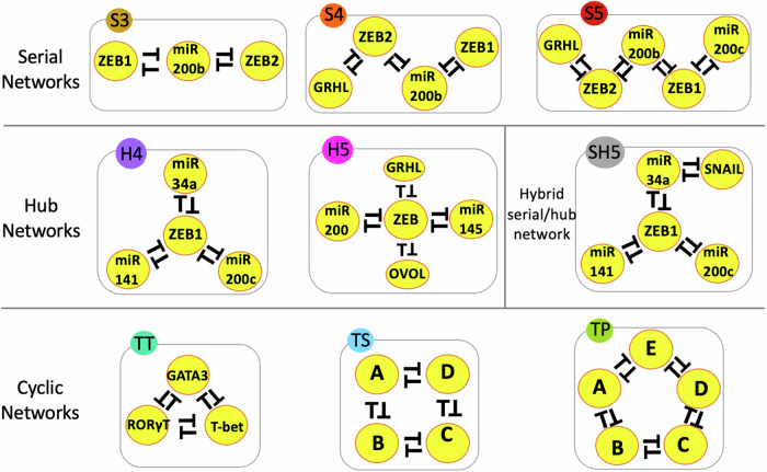
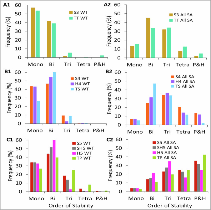
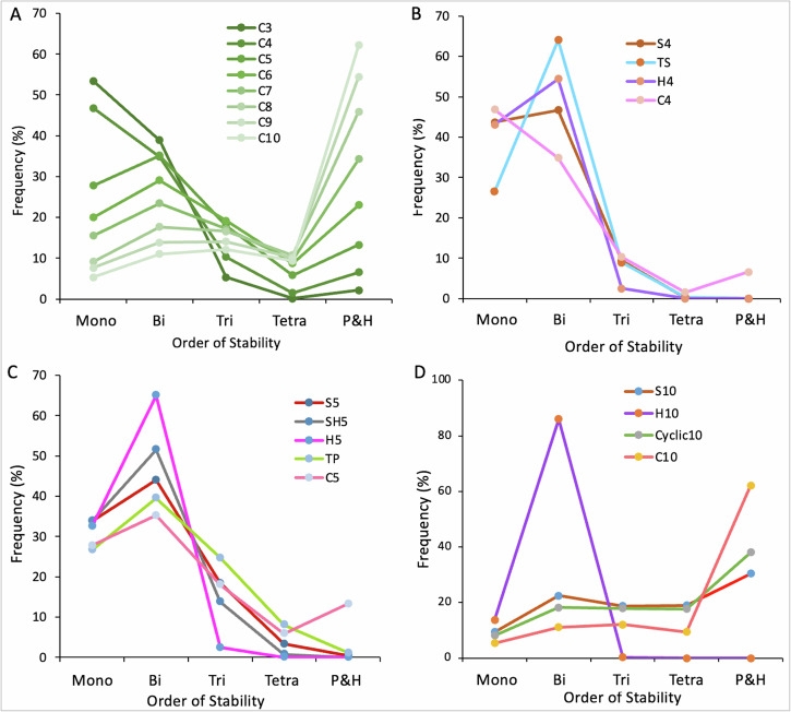
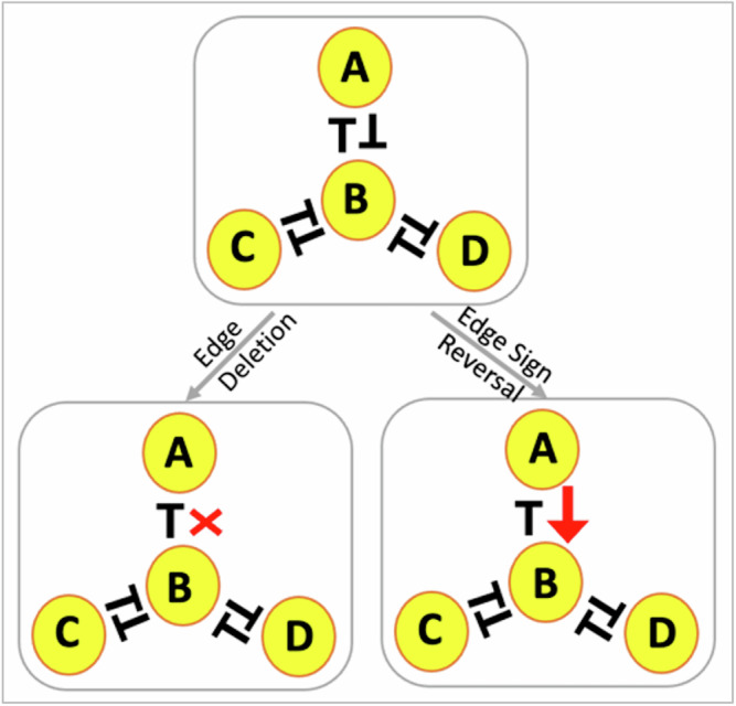
Interconnected feedback loops are prevalent across biological mechanisms, including cell fate transitions enabled by epigenetic mechanisms in carcinomas. However, the operating principles of these networks remain largely unexplored. Here, we identify numerous interconnected feedback loops implicated in cell lineage decisions, which we discover to be the hallmarks of lower- and higher-dimensional state space. We demonstrate that networks having higher centrality nodes have restricted state space while those with lower centrality nodes have higher dimensional state space. The topologically distinct networks with identical node or loop counts have different steady-state distributions, highlighting the crucial influence of network structure on emergent dynamics. Further, regardless of topology, networks with autoregulated nodes exhibit multiple steady states, thereby "liberating" network dynamics from absolute topological control. These findings unravel the design principles of multistable networks implicated in fate decisions and can have crucial implications in engineering or comprehending multi-fate decision circuits.

Fig. 1. Schematics of high-dimensional feedback loops.

In serial networks, multiple toggle switches are connected end-to-end. In hub networks, multiple nodes interact with a common node. In cyclic networks, a closed loop is formed between the network nodes. Each network is assigned a unique color code for comparative analysis and a name reflecting the type of topology and the number of nodes in the network. For instance, S3 is a Serial network with three nodes, and H4 is a Hub network with four nodes, and so on. SH5 has a hybrid Serial-Hub (SH) topology with five nodes. The toggle triad (TT), toggle square (TS), and toggle polygon (TP) networks have cyclic topologies with three, four, and five nodes, respectively. Networks with annotated nodes are real biological networks and those without annotations are “synthetic” networks. Lines with a bar denote inhibition/repression. Mutual inhibition between two nodes forms a toggle switch.

Fig. 2. Distribution of stable steady states for serial and hub networks.

The SSD of wild-type serial and hub networks (A) and their self-activated (SA) counterparts (B). Gene expression data projected on the 1st and 2nd principal component axis for WT networks (C) and their self-activated counterparts (D). Each dot (of 10,000 dots) in the plot is a stable steady state (or phenotype) of a model corresponding to a specific parameter set. K-means clustering was used to group locally identical states and identify distinct “global” states that represent distinct cell states (phenotypes) a network can support (see methods for details). The number of phenotypes increase as network size increases serially (say, from S3 to S5) and remains unchanged as network size increases and becomes hub (say, from S3 to H4 to H5). Mono, Bi, Tri, and Tetra denote monostable, bistable, tristable, and tetrastable states. Penta-and higher (P&H) collectively denotes five and up to ten states, respectively. “WT” implies a wild-type (without any perturbation) network. “All SA” means all nodes are self-activated. “X” in scatter plots denotes the centroids of the clusters. Cluster colors have no correspondence with the colors used to designate networks.

Fig. 3. SSD comparison of topologically distinct networks having an equal number of nodes.

A1 Three-node networks showing almost overlapping SSD. B1 Four-node networks show non-overlapping SSD. Cyclic network TS functions like a serial network S3, in the sense that both tend to exhibit higher-order stabilities as compared to H4. C1 Five-node networks again show non-overlapping bi-and higher-order (tristable and above) SSD. The cyclic network TP functions like a serial network with more frequent higher-order steady states. Except in (A1), the same node-count networks in (B1, C1) show variable SSD. A2, B2, C2 Self-activated counterparts of networks in (A1–C1), show that self-activated networks with the same node count have comparable SSD as compared to their WT counterparts.

Fig. 4. SSD comparison of topologically distinct networks having an equal number of toggle switches.

A1 Networks with three toggle switches have non-overlapping SSD. Despite having one node less than H4, cyclic network TT still shows some possibility for tristability. B1 Four-node networks again show non-overlapping higher-order SSD. Again TS, despite having one node less than H5, has greater tristable frequencies showing that cyclic network TS functions like a serial network by supporting higher-order steady-states. A2, B2 Self-activated counterparts of networks in (A1, B1).

Fig. 5. Comparative analysis of the steady state distribution in complete networks.

A Complete networks with three to ten nodes. B Comparison of a four-node complete network, C4, with all four-node networks. C Comparison of a five-node complete network, C5, with all five-node networks. D Comparison of a ten-node complete network, C10, with ten-node serial (S10), hub (H10), and cyclic (cyclic10), networks.

Fig. 6. Illustration of the two types of network perturbations.

An unperturbed network (WT) with ED and ESR perturbations. In ED, one of the edges between the two nodes is deleted, resulting in a breakdown of the positive feedback loop. In ESR, the sign of one of the edges between the two nodes is changed from inhibition to activation so that a positive feedback loop transforms into a negative feedback loop. The lines with a bar denote inhibition/repression and those with an arrow denote activation.

Fig. 7. Effect of two types of edge perturbations, ED and ESR, on the SSD of SH5 (representative network).

A In a non-autoregulated (without self-activations) network, an ESR increases monostable states more rapidly than an ED. B The effect of edge perturbations is diluted by the self-activations as the differences in SSD between WT and its two perturbed counterparts are negligible. Gene expression data of WT (C) and SA (D) networks projected on the 1st and 2nd principal component axis after clustering. Each cluster represents the steady state of a network state. SH5 WT means SH5 unperturbed network, 1ED means one edge detection, 1ESR means one edge sign reversal, and all-SA means all nodes are self-activated.

Fig. 8. Effect of multiple ED and ESR perturbations on multistability.

The plots illustrate the effect of increasing EDs and ESRs on the emergent SSD of HDFLs by considering SH5 as a representative network. A As EDs increase, the frequency of monostable states increases while bi-and-tri stable states decrease proportionately. Deleting three edges (breaking three PFLs) increases the frequency of monostable states to nearly 80% from nearly 30% in WT while also removing the chance of occurrence of any tristable solution. A completely monostable dynamics is achieved upon breaking all four PFLs in SH5. B As ESRs increase, network dynamics shift to mono-and-bistability faster than in the case of each ED. The 80:20 ratio of monostable: bistable states is achieved with two ESRs (i.e., converting two PFLs to NFLs) compared to three EDs and the frequency of tristable states is almost negligible. A completely monostable dynamics is achieved by converting four PFLs to NFLs. Gene expression data of SH5 with 4EDs (C) and 4ESR (D) projected on the 1^st and 2^nd principal component axis after clustering. A cluster represents a single state state. WT denotes no ED or ESR and 4ED (4ESR) denotes four edge deletions (edge sign reversals).

Fig. 9. Bar plots showing the importance of the position of edge perturbations in networks with- and without self-activated nodes.

A A non-self-activated (WT) S3 network and its two ED perturbations. B Same as (A) but with ESRs. C S3 network with one of the terminal nodes self-activated and its two ED perturbations. (D) same as (C) but with ESRs. Perturbations, P1 and P2, are done in two toggle switches on the opposite sides of the central node of S3 so that in (C, D), P1 involves the SA node while P2 doesn’t. 1EDP1/1EDP2 (1ESRP1/1ESRP2) denote single-edge deletions (edge sign reversals) at P1 and P2 position. This terminology follows throughout the bar plots in Fig. S8.

Fig. 10. Bifurcation diagrams for the steady states of gene x₁ with respect to its basal production rate, B₁.

Top panel: three serial networks, S3, S4, and S5. Bottom panel: single edge deleted S3 network, hub network H5, and cyclic network, TP. Solid curves represent stable steady states, and dashed curves represent unstable steady states. In S3, S4, S5, and H5 networks, $x_1$ represents ZEB1, GRHL, GRHL, and miR200, respectively. In TP network $x_1$ represents node A. The colors of the stable branches of the bifurcation diagrams are matched to the color codes of the networks in Fig. 1. The model system (4) was used for the bifurcation analysis of S3, S4, and S5 networks. The model systems for H5 and TP networks and the parameters for all models are listed in Supplementary Information, Section S9. Bifurcations were generated using custom MATLAB codes.

References

1. Jia, D., Jolly, M. K., Kulkarni, P. & Levine, H. Phenotypic Plasticity and Cell Fate Decisions in Cancer: Insights from Dynamical Systems Theory. Cancers9, 70 (2017). - PMC - PubMed
1. Levine H. et al. Decoding the mechanisms underlying cell-fate decision-making during stem cell differentiation by random circuit perturbation. 10.1098/rsif.2020.0500 (2020). - PMC - PubMed
1. Brown, M. S. et al. Phenotypic heterogeneity driven by plasticity of the intermediate EMT state governs disease progression and metastasis in breast cancer. Sci. Adv.8, eabj8002 (2022). - PMC - PubMed
1. Moris, N., Pina, C. & Martinez Arias, A. Transition states and cell fate decisions in epigenetic landscapes. 10.1038/nrg.2016.98 (2016). - PubMed
1. Zhou, J. X. & Huang, S. In press. Understanding gene circuits at cell-fate branch points for rational cell reprogramming. 10.1016/j.tig.2010.11.002 - PubMed
MeSH terms
LinkOut - more resources