High-resolution genomic history of early medieval Europe

Abstract

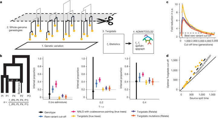
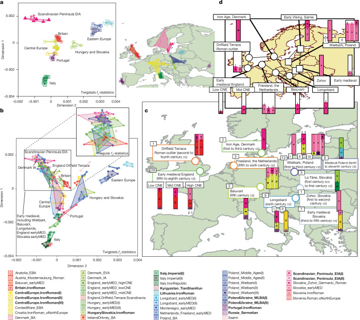
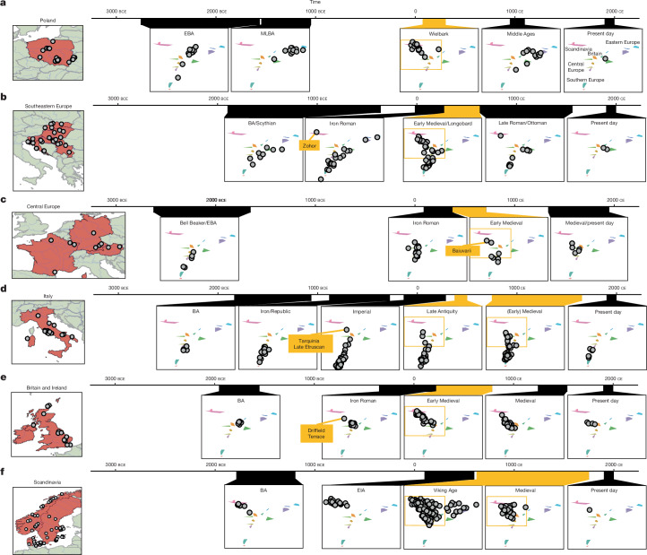
Many known and unknown historical events have remained below detection thresholds of genetic studies because subtle ancestry changes are challenging to reconstruct. Methods based on shared haplotypes^1,2 and rare variants^3,4 improve power but are not explicitly temporal and have not been possible to adopt in unbiased ancestry models. Here we develop Twigstats, an approach of time-stratified ancestry analysis that can improve statistical power by an order of magnitude by focusing on coalescences in recent times, while remaining unbiased by population-specific drift. We apply this framework to 1,556 available ancient whole genomes from Europe in the historical period. We are able to model individual-level ancestry using preceding genomes to provide high resolution. During the first half of the first millennium CE, we observe at least two different streams of Scandinavian-related ancestry expanding across western, central and eastern Europe. By contrast, during the second half of the first millennium CE, ancestry patterns suggest the regional disappearance or substantial admixture of these ancestries. In Scandinavia, we document a major ancestry influx by approximately 800 CE, when a large proportion of Viking Age individuals carried ancestry from groups related to central Europe not seen in individuals from the early Iron Age. Our findings suggest that time-stratified ancestry analysis can provide a higher-resolution lens for genetic history.

Fig. 1. Twigstats performance on simulated data.

a, A diagram of the Twigstats approach. We first construct genealogies from genetic variation data and then use Twigstats to compute f₂-statistics between pairs of groups to be used by ADMIXTOOLS2. b, Admixture proportions inferred from an f₄-ratio statistic or non-negative least squares method. Source groups P1 and P2 split 250 generations ago and mix 50 generations ago, where P2 contributes proportion α and P1 contributes 1 − α. Effective population sizes are equal and constant except for a recent bottleneck in P2 (see Methods for simulation details). The Twigstats cut-off is set to 500 generations, the rare variant cut-off is set to 5%, and we additionally infer admixture proportions by generating ‘first coalescence profiles’ for each population and modelling PX as a mixture of sources P1 and P2 using non-negative least squares (NNLS) (Methods). We sample 20 haploid sequences from each population. Data are mean ± 2 s.e. around the point estimate. c, The fold improvement of s.e. relative to the genotype case as a function of the Twigstats cut-off time, for the same simulation as in b and averaged across different true admixture proportions. The dashed line shows the best fold improvement of s.e. when ascertaining genotypes by frequency, when evaluated at different frequency cut-offs. d, The optimal Twigstats cut-off, defined as the largest reduction in s.e. relative to the genotype case, as a function of source split time in simulations using true trees. The dashed line indicates our theoretical prediction (Supplementary Note).

Fig. 2. Ancestry from the Iron Age to the early medieval period in Europe.

a, Source groups used for qpAdm modelling of early medieval Europe. MDS is computed jointly with individuals from later periods using pairwise outgroup f₃ statistics (outgroup: Han Chinese people). These are calculated using Twigstats on Relate genealogies with a cut-off of 1,000 generations. The geographical map shows sampling locations of these individuals. b, The genetic structure of ancient groups predominantly from early medieval contexts shown on the same MDS as in a. The magnified inset shows an MDS computed without Twigstats on the same samples as the Twigstats MDS and focusing on early medieval or later individuals. c, Ancestry models of early medieval (EM) groups across Europe computed using qpAdm. Sample sizes are shown in black boxes. Sources are highlighted in a and marked as bold in the key, and were used in a rotational qpAdm scheme. For each target group, we remove models with infeasible admixture proportions (falling outside [0, 1]) and use a Twigstats cut-off of 1,000 generations. All models satisfy P > 0.01, unless a −log₁₀[P value] is shown next to the model. If models satisfy P > 0.05, we show all such models; otherwise, we show only the model with the largest P value. d, The ancestry proportion derived from EIA Scandinavia in groups with a non-zero component of this ancestry. We show groups modelled in c that have a feasible model (P > 0.01). In c,d, we show one s.e. BA, Bronze Age; CNE, continental northern Europeans; EBA, early Bronze Age; EVA, early Viking Age; IA, Iron Age; MED, medieval; MLBA, middle/late Bronze Age; VA, Viking Age.

Fig. 3. Time transects across six geographical regions in Europe.

a–f, Ancestry change visualized over a time transect spanning from the Bronze Age to the present day in Poland (a), southeastern Europe (b), central Europe (c), Italy (d), Britain and Ireland (e) and Scandinavia (f). The maps show sample locations of all available ancient genomes with at least 0.5× coverage from these regions (Supplementary Table 1). Their ancestry is shown on the same MDS model as in Fig. 2a for each time period. For each geographic region, the early medieval period is highlighted in orange and the area in the MDS corresponding to Scandinavian and central European ancestries is highlighted in an orange box.

Fig. 4. Ancestry in the Viking world.

a, Map showing ancestry carried by Scandinavian Viking Age individuals as inferred using the best-fitting qpAdm model. These are chosen by either choosing the one-source model with largest P value and P > 0.01 or the two-source model with the largest P value and P > 0.01. Extended Data Fig. 7 shows the same map with all accepted models. b, Stable isotope data indicating the geology of childhood origin. The histogram shows the ratio of strontium isotopes 87 to 86 measured in 109 individuals in Öland. For individuals included in our ancestry modelling, we plot Iron Age central European-related ancestry against their stable isotope values (grey circles, r = −0.39, P = 0.075). Shared area corresponds to the 95% confidence band around the regression line. c, The ancestry shift observed in Viking Age Danish groups using qpAdm on all SNPs or Twigstats. We show the best one-source and all two-source models with P > 0.05. For models with P < 0.05, the −log₁₀[P value] is shown under the plot. Sample sizes for each group are shown in brackets. d, The ancestry proportion across Viking Age individuals in Denmark, Sweden and Norway grouped by latitude. e, Viking Age genetic variation (grey circles) visualized on the same MDS as in Fig. 2a,b. f, The best-fitting qpAdm ancestry model for far-flung Viking individuals. Detailed models for all individuals are shown in Extended Data Figs. 9 and 10. In c and f, we show one s.e. Rotating qpAdm sources are marked in bold in the key.

Extended Data Fig. 1. Collection of ancient genomes used in this study.

a, Ancient DNA samples included in this study (Supplementary Table 1). Samples older than 3000 BCE are shown at 3000 BCE. b, Map showing mean coordinates of groups in the Iron, Early Modern, and Viking Ages. c, Source groups used in qpAdm modelling of Metal Age and early Medieval Europe (Figs. 2, 3 and 4), showing sample ages. Sample sizes are shown in grey boxes. d, F_ST between Metal Age and early Medieval groups computed using popstats using options --FST --informative. Sample sizes are shown in brackets and we show one standard error.

Extended Data Fig. 2. Twigstats optimal cutoff.

a, Theoretically computed z-score of f₄(PO,P1,PX,P2) at a single genomic locus (Supplementary Note), assuming PX is admixted between P1 and P2 at time 0.004 (in units of 2N_e generations), e.g. corresponding to 100 generations with 2N_e of 25,000. Sources split at time 0.02. b, The theoretical fold-improvement of the best Twigstats z-score of f₄(PO,P1,PX,P2) relative to the z-score obtained with regular f₄-statistics. We use the same parameters as in a, but vary source split times to illustrate the improved power for mixtures involving more closely related groups. c, The optimal Twigstats cutoff time as a function of the source split time and the ratio between the optimal cutoff time and source split time. d, Comparison of z-scores computed using Twigstats to the corresponding theoretical values shown in a.

Extended Data Fig. 3. Simulations.

a, Theoretically computed r² stratified by minor allele frequency between true genotypes and genotypes with randomly introduced errors (Methods), emulating imputation accuracy plots. b, Admixture simulation where sources P1 and P2 split 250 or 500 generations ago and a pulse admixture event gives rise to a target population PX 50 generations ago. We vary demographic history, error rates, and sample sizes and simulate 20 replicates for each scenario (see Methods for simulation details). Admixture proportions are computed using an f₄-ratio statistic and the Twigstats cutoff is set to twice the source split time and the rare variant cutoff is 5%. We plot two standard errors around the mean. c, qpAdm simulation taken from^,, as well as an adapted version where all population split times and the admixture date are divided by 5. The Twigstats cutoff time is chosen to be 1200 generations (top) and 600 generations (bottom). We simulate 10 replicates and plot two standard errors around the mean. d, Simulation adapted from of a stepping stone model with 9 populations organised on a 1-dimensional grid as shown, where individuals are able to migrate between adjacent fields. We run a rotational qpAdm to fit population 4 using other pairs of populations to the left and right as sources. We run 50 replicates and set the p-value of models with inferred proportions outside of [0,1] to 0. We then compute the proportion where a given pair achieves the best p-value (top) and show the median p-value across these replicates (bottom). In all simulations in b, c, d, we sample N = 20 haploid sequences per population, except for one simulation in b, where we sample N = 100 sequences.

Extended Data Fig. 4. Relationship of mutation age and MAF.

a, Heatmap showing the distribution of mutation ages for each minor allele frequency (MAF) bin. To account for the uncertainty in when the mutation arose on a branch, we sample a random date between the lower and upper ends of the branch onto which it maps. We use 20 replicates of the simulation of Fig. 1b, where sources split 500 generations ago and the admixture proportion is 0%. b, Same as a but using mutation ages determined by Relate-inferred genealogies. We place mutations at the same relative height between the lower and upper ends of a branch as in the true trees to remove the uncertainty in when on the branch the mutation occurred, so that we would recover the true allele age from a correctly inferred genealogy. c, Pearson correlation between MAF, true mutation age, and Relate mutation ages, as well as the same comparisons when restricting to mutations of MAF less than 0.1.

Extended Data Fig. 5. Three examples of applying Twigstats.

a Fine-scale population structure simulation emulating ref. (see Methods for simulation details). First two principal components are computed from pairwise outgroup f₃ statistics on the genotypes directly and on Relate trees inferred from the 50 target individuals. Labels in plots show the average coordinates of members of that population. For each panel, we calculate a separation index (SI) as in, which we define as the proportion of individuals for which the closest individual (by the Euclidean distance in PC space) is in the same population. b, Fine-scale genetic structure in Neolithic Europe quantified using an MDS calculated on a symmetric matrix that contains all pairwise outgroup f₃ statistics (outgroup: YRI) between individuals. These are either calculated directly on genotypes or calculated using Twigstats on Relate genealogies with a cutoff of 1000 generations. Individuals were selected by filtering based on Steppe and Western Hunter-gatherer ancestry (Methods). c, Admixture proportions inferred using qpAdm with three distal sources of Western Hunter-gatherers, early European farmers, and Yamnaya Steppe people. We show results for Twigstats-5000. Bias is measured as the difference in admixture proportions obtained from Twigstats-5000 and all SNPs, and we show standard errors of the latter. We plot two standard errors around the mean. The standard error improvement shown is one minus the ratio of standard errors obtained from Twigstats-5000 and using all SNPs. d, Neanderthal admixture proportion inferred using an f₄-ratio of the form f₄(outgroup, Altai, target, Mbuti)/f₄(outgroup, Altai, Vindija, Mbuti). We compute these on genetic variation data from the Simon’s Genome Diversity Project (SGDP) and use the high-coverage Altai and Vindija Neanderthals^,. We also compute equivalent f₄-ratio statistics in a simulation emulating Neanderthal admixture 50,000 years ago and a second simulation involving no Neanderthal admixture but deep structure that leads to a similar inference unless deep coalescences are ignored by Twigstats. We plot two standard errors around the mean.

Extended Data Fig. 6. MDS of ancient and modern genomes.

a, Same MDS as in Fig. 2 but only showing qpAdm source groups of Fig. 2a and modern groups in the Simons Genome Diversity Project (labelled) computed using genotypes (top) or Twigstats (bottom). b, MDS computed using genotypes showing one early medieval or Viking age group per facet. c, MDS computed using Twigstats showing one early medieval or Viking age group per facet.

Extended Data Fig. 7. Ancestry estimates stratified by genetic sex.

a, Map showing ancestry carried by each Scandinavian Viking age individual. b, Ancestry proportions across individuals grouped by Latitude and genetic sex. c, Odds ratio and p-values calculated using a two-sided Fisher’s exact test on the number of males and females carrying each ancestry in Viking Age Denmark, Sweden, Norway, Iceland, and Gotland. d, F₄ values of the form f₄(Scandinavian_Peninsula_EIA(I), alternative source group, males in Viking group, females in Viking group) computed using all SNPs and Twigstats. A significantly positive value is evidence of attraction of females with pop2 or males with Scandinavian_Peninsula_EIA(I). Number of males and females is shown in each facet title and we restrict to groups with at least four males and females. We plot one standard error. e, Map showing ‘farflung’ Viking individuals grouped by ancestry and genetic sex. In contrast to Fig. 4a and d where we showed results for the ‘best’ qpAdm model, here in panels a, b, c, and e, an individual is assigned an ancestry group, if it has any accepted model (p > 0.01) where that ancestry features.

Extended Data Fig. 8. Replication previous Viking Age ancestry modelling.

a, P-values of 1-source qpAdm models with target groups shown as rows and source groups shown as columns, replicating Extended Data Fig. 5a of ref. Left column uses p-values obtained from ref. . Middle and right column correspond to newly computed p-values in a qpAdm using, respectively, all SNPs and Twigstats-2000. Outgroups are YRI, CHB, DevilsCave_N.SG, WHG, EHG, Anatolia_N, Yamnaya, Estonia_CordedWare.SG (Supplementary Table 1). We excluded Denmark_IA.SG and England_Roman.SG from the rotational scheme as these groups overlap in ancestry with England_IA.SG and Norway_IA, respectively. Only samples with coverage exceeding 0.5 are used. For each target group, the source group with the largest p-value is shown with a black circle. b, qpAdm models of ref. where modern populations are used as sources. As in ref. , we show ancestry proportions averaged over individuals in each group, where for each individual the model with the smallest number of sources and largest p-value is chosen. c, Replication using the same target samples as in b. We fit a maximum of two sources and choose the model with the smallest number of sources and largest p-value, requiring p > 0.01 for 1 source and p > 0.001 for 2 source models. The set of individuals used in b and c are identical and are comprised of targets with an accepted model in all SNPs and Twigstats-1000, removing 15 of 167 individuals. We additionally remove 17 individuals that did not have a feasible model in ref. .

Extended Data Fig. 9. Ancestry models of Viking Age individuals in Scandinavia.

a, MDS of each Scandinavian Viking group plotted on top of preceding Iron age and Roman individuals. b, All accepted qpAdm models using Twigstats-1000 for every Scandinavian Viking individual in Denmark, Sweden, and Norway, computed in a rotational qpAdm with source groups identical to Fig. 4. We only retain models with feasible admixture proportions, standard errors of <0.25, and show models with 1 source and a p-value greater than 0.01 or otherwise with 2 sources and a p-value greater than 0.01. If several models satisfy p > 0.05, we show all such models, otherwise we select the model with the largest p-value. The -log10 p-values are shown to the left of each model. We combine models involving related sources, if they exist, by averaging their respective admixture proportions, standard errors, and p-values. We plot one standard error.

Extended Data Fig. 10. Ancestry models of farflung Viking individuals.

a, MDS of each farflung Viking group plotted on top of preceding Iron age and Roman individuals. b, All accepted qpAdm models using Twigstats-1000 for every non-Scandinavian Viking individual computed in a rotational qpAdm with source groups identical to Fig. 4. We plot one standard error.

References

1. Lawson, D. J., Hellenthal, G., Myers, S. & Falush, D. Inference of population structure using dense haplotype data. PLoS Genet.8, 11–17 (2012). - PMC - PubMed
1. Hellenthal, G. et al. A genetic atlas of human admixture history. Science343, 747–751 (2014). - PMC - PubMed
1. Schiffels, S. et al. Iron Age and Anglo-Saxon genomes from East England reveal British migration history. Nat. Commun.7, 10408 (2016). - PMC - PubMed
1. Flegontov, P. et al. Palaeo-Eskimo genetic ancestry and the peopling of Chukotka and North America. Nature570, 236–240 (2019). - PMC - PubMed
1. Antonio, M. L. et al. Stable population structure in Europe since the Iron Age, despite high mobility. eLife13, e79714 (2024). - PMC - PubMed
LinkOut - more resources