Decomposition of the pangenome matrix reveals a structure in gene distribution in the Escherichia coli species

Abstract

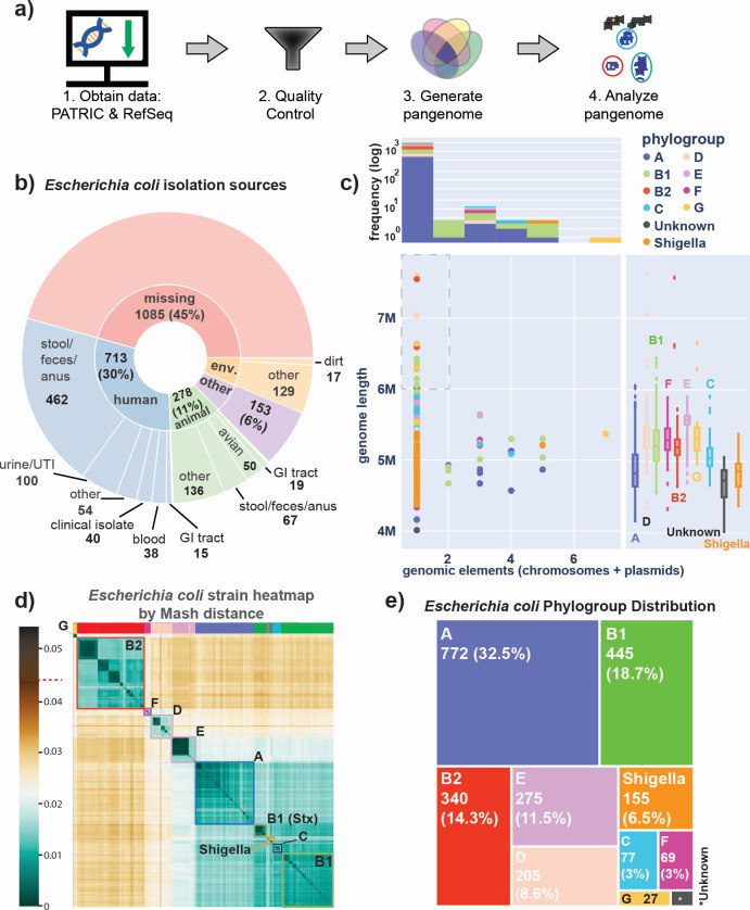
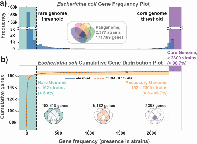
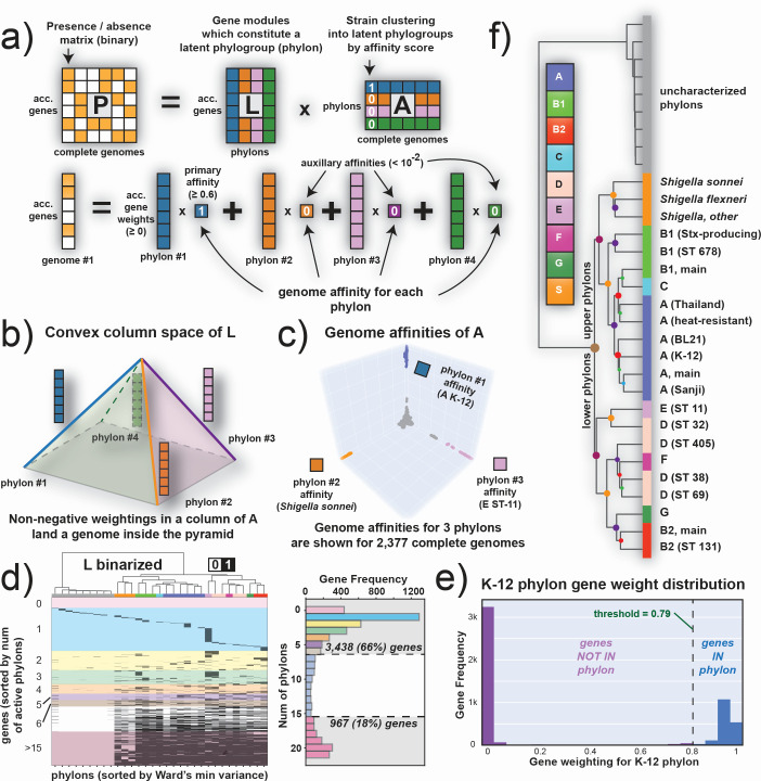
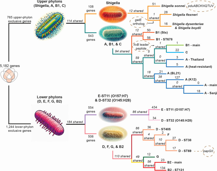
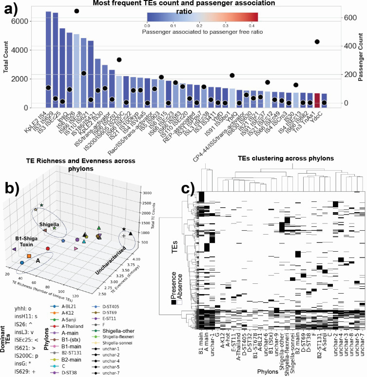
Thousands of complete genome sequences for strains of a species that are now available enable the advancement of pangenome analytics to a new level of sophistication. We collected 2,377 publicly available complete genomes of Escherichia coli for detailed pangenome analysis. The core genome and accessory genomes consisted of 2,398 and 5,182 genes, respectively. We developed a machine learning approach to define the accessory genes characterizing the major phylogroups of E. coli plus Shigella: A, B1, B2, C, D, E, F, G, and Shigella. The analysis resulted in a detailed structure of the genetic basis of the phylogroups' differential traits. This pangenome structure was largely consistent with a housekeeping-gene-based MLST distribution, sequence-based Mash distance, and the Clermont quadruplex classification. The rare genome (consisting of genes found in <6.8% of all strains) consisted of 163,619 genes, about 79% of which represented variations of 315 underlying transposon elements. This analysis generated a mathematical definition of the genetic basis for a species.

Importance: The comprehensive analysis of the pangenome of Escherichia coli presented in this study marks a significant advancement in understanding bacterial genetic diversity. By employing machine learning techniques to analyze 2,377 complete E. coli genomes, the study provides a detailed mapping of core, accessory, and rare genes. This approach reveals the genetic basis for differential traits across phylogroups, offering insights into pathogenicity, antibiotic resistance, and evolutionary adaptations. The findings enhance the potential for genome-based diagnostics and pave the way for future studies aimed at achieving a global genetic definition of bacterial phylogeny.

Keywords: Escherichia coli; Shigella; computational biology; genome analysis; genomics; typing.

Fig 1

Processing and classification of a 2,377 complete Escherichia coli genome compendium (GENOMiCUS). (a) The workflow used in this study. Genomes were downloaded from PATRIC (now BV-BRC) and RefSeq, after which they were deduplicated and filtered based on their quality metrics (see Methods). The resulting 2,377 complete genomes form a high-quality compendium of strains for detailed pangenome analysis. We call this compendium the Genome Encyclopedia of Notable Observed MIcro-organisms Curated for Universal Study (GENOMiCUS). (b) A sunburst plot showcasing the different isolation sources for the bacteria in this compendium. While most of the 1,332 isolation site-annotated strains come from humans (713), there are many strains isolated from animals (278) and various other environmental niches (146). (c) Scatterplot summarizing properties of the genomes by genome length (y-axis) vs number of genomic elements (chromosomes + plasmids) (x-axis), colored by phylogroup as calculated in silico by the ClermonTyping github package (18). Note that many Shigella strains were incorrectly classified by ClermonTyping as belonging to Phylogroup A, and so any strains which were known to be Shigella were manually separated into a separate class for better identification. Nineteen strains were found to have a genome size greater than 6 Mb. Sixteen of those 19 strains were clinical isolates from ICDDR,B from patients who had diarrheal disorders. Above the scatterplot is a histogram showcasing the genomic element distribution within the strains of the pangenome, also colored by phylogroup. Note: in this context, a “genomic element” refers to both the main chromosome and any additional plasmids found in the organism. To the right of the scatterplot are phylogroup-specific boxplots describing the distribution of genome lengths per phylogroup. (d) A heatmap of the pairwise Mash distances for all 2,377 E. coli strains of GENOMiCUS based on sequence analysis. Distances range from 0 to 0.04, and the highest Mash value (0.044) is denoted with a red dash on the color bar. Note that a pairwise Mash distance of 0.05 equates to an average nucleotide identity (ANI) of 95%, both of which correspond to a 70% DNA–DNA reassociation value, the historical definition of a bacterial species (19, 20). The highlighted bars at the top of the heatmap identify the Mash-based clusters of this compendium. Phylogroups are annotated on the heatmap, showing the correspondence between these phylogroups and the Mash-based clusters. (e) Treemap illustrating the distribution of E. coli strains by phylogroup as calculated in silico by the ClermonTyping github package (18).

Fig 2

Global distributions of gene frequencies and functions in the Escherichia coli pangenome. (a) Gene frequency distribution across the 2,377 curated genomes in GENOMiCUS. Genes present in all 2,377 strains appear at the histogram’s right end. Progressing leftward, subsequent bars show genes found in nearly all strains, decreasing in frequency, until reaching genes unique to just one strain at the extreme left. (b) The cumulative gene distribution function (23). The gene frequency distribution was fitted to a double-exponential form (with median absolute error or MAE = 176.31) and the inflection points determined. Based on these inflection points, the genes in the pangenome were divided into the core (comprising 2,398 genes), accessory (comprising 5,182 genes), and rare (comprising 163,619 genes) genomes (See Methods).

Fig 3

The fundamental mathematical structure of the E. coli accessory genome. Characteristics of the NMF decomposition of the pangenome matrix P. (a) A column of P (i.e., genome #1) is a linear combination of the phylon vectors as determined by the weights in the corresponding column of A. (b) Since the phylon vectors are non-negative, they span a polygon as its edge vectors. A positive linear combination of the L_i vectors lands inside the polygon. (c) Since there is typically only one dominant value in a column of A, the reconstruction of a column in P (i.e., one genome) lies close to a phylon vector (i.e., the edges of the polygon) as is evident for the 2,377 sequenced strains used. (d) A clustermap of the binarized L matrix. Colors on top correspond with classically defined phylogroups as determined by ClermonTyping. Columns are clustered using Ward’s minimum variance method, and rows are sorted by gene frequency in each phylon (i.e., genes in zero phylons are at the top, genes in 22 phylons are at the bottom). The dendrogram at the top of L, showing the clustering of its columns, is the same as that used in panel (f). In this graphical representation the black elements designate that the gene responding to that row is found in the phylon that the column represents. White elements mean that the corresponding gene is not found in the phylon. The histogram to the right of the clustered L matrix showcases the gene frequency across multiple phylons (i.e., how many phylons a gene is present in). The colors in L-binarized correspond to the colors on this histogram and showcase the distribution of genes by their number of active phylons; 3,438 (66%) of the 5,182 accessory genes are found in six or fewer phylons, with the plurality being genes active in only one phylon (1,289 single-phylon genes, 25% of all 5,182 accessory genes). (e) A gene weight distribution for one particular phylon consisting of K-12 strains in the L matrix. Most genes have a weighting close to zero, with a notable cluster having weightings between 0.8 and 1. The genes with low weightings (below the threshold indicated by the dashed line) are binarized to zero and considered not to be part of the phylon, while genes with high weightings are binarized to one and considered to be constituents of this phylon. The threshold for binarization is determined for each phylon using k-means clustering (see Methods). (f) A dendrogram of all 31 phylons based on clustering the binarized L matrix shown in panel (d). The uncharacterized phylons are separated, mainly consisting of phage genes and other mobile elements.

Fig 4

A clustering diagram of the phylons (see Fig. 3f) that highlights the groups of exclusive genes that follow one branch and not the other at each branch point. The numbers above the line leading to a split indicate exclusive genes (i.e., genes found in one group of phylons but absent in the other). Numbers in italics specifically indicate shared genes that are found across all groups. The function and identity of special genes of interest are discussed in the main text, and detailed in Table S2. Four specific genetic traits of interest are highlighted in dashed ovals, such as the papGII operon to phylon D (ST69). This sequence variant of papG in this operon is associated with UTIs that can become bacteremic (28, 29).

Fig 5

Transposable elements (TEs) in the rare genome. (a) Frequency of the 40 most abundant TEs of the 315 TE types found in the pangenome, and the ratio of passenger-free to passenger-associated TEs. Bar plot represents count of each group of TEs (top x-axis), bar color indicates the ratio of passenger-free TEs to passenger-associated TEs, and dots indicate the count of passenger genes associated with each group of TEs (bottom x-axis). Naming convention of the TEs is derived from PROKKA annotation. (b) Phylon TEs count, richness, and entropy; colors represent phylons, signs indicate the dominant TE found in each phylon, TE richness shows how many unique types of TE inhabited a phylon, TE evenness shows how evenly a phylon is infected with different types of TE, higher values of evenness indicates greater entropy. Phylons with fewer than 30 genomes were excluded from the analysis. For phylons with more than 30 genomes, a random subset of 30 genomes was selected, and the remaining genomes were excluded (Fig. S5c illustrates the sensitivity of TE richness, evenness, and count metrics to the random sampling of genomes); the symbols on the plot represent the dominant TE in each phylon: circle ('o') for yhhI, square (’s') for insH11, upward triangle ('^') for IS26, downward triangle ('v') for insL3, left-pointing triangle ('<') for ISEc25, right-pointing triangle ('>') for IS621, pentagon ('p') for IS200C, star ('*') for insG, and plus ('+') for IS629. (c) Represents a heatmap generated using CD-HIT clustering results, depicting the distribution of TEs across various phylons. Each cell in the heatmap represents the presence (black) or absence (white) of a specific group of TEs in a given phylon. The hierarchical clustering, employing the Ward method, is applied both horizontally and vertically, illustrating the grouping of similar TEs and phylons, respectively. The dendrograms adjacent to the rows and columns indicate the clustering relationships.

References

1. Fleischmann RD, Adams MD, White O, Clayton RA, Kirkness EF, Kerlavage AR, Bult CJ, Tomb JF, Dougherty BA, Merrick JM. 1995. Whole-genome random sequencing and assembly of Haemophilus influenzae Rd. Science 269:496–512. doi:10.1126/science.7542800 - DOI - PubMed
1. Blattner FR, Plunkett G 3rd, Bloch CA, Perna NT, Burland V, Riley M, Collado-Vides J, Glasner JD, Rode CK, Mayhew GF, Gregor J, Davis NW, Kirkpatrick HA, Goeden MA, Rose DJ, Mau B, Shao Y. 1997. The complete genome sequence of Escherichia coli K-12. Science 277:1453–1462. doi:10.1126/science.277.5331.1453 - DOI - PubMed
1. Perna NT, Plunkett G III, Burland V, Mau B, Glasner JD, Rose DJ, Mayhew GF, Evans PS, Gregor J, Kirkpatrick HA, et al. . 2001. Genome sequence of enterohaemorrhagic Escherichia coli O157:H7. Nature 409:529–533. doi:10.1038/35054089 - DOI - PubMed
1. Kris A. Wetterstrand MS. 2019. The cost of sequencing a human genome. NHGRI. Available from: https://www.genome.gov/about-genomics/fact-sheets/Sequencing-Human-Genom.... Retrieved 18 Apr 2023.
1. Olson RD, Assaf R, Brettin T, Conrad N, Cucinell C, Davis JJ, Dempsey DM, Dickerman A, Dietrich EM, Kenyon RW, et al. . 2023. Introducing the Bacterial and Viral Bioinformatics Resource Center (BV-BRC): a resource combining PATRIC, IRD and ViPR. Nucleic Acids Res 51:D678–D689. doi:10.1093/nar/gkac1003 - DOI - PMC - PubMed