A spatial code for temporal information is necessary for efficient sensory learning

Abstract

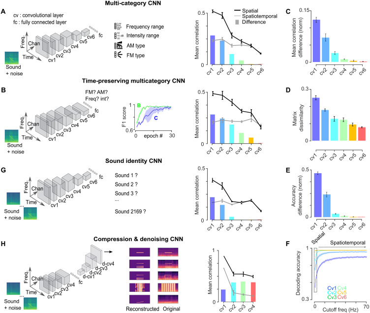
The temporal structure of sensory inputs contains essential information for their interpretation. Sensory cortex represents these temporal cues through two codes: the temporal sequences of neuronal activity and the spatial patterns of neuronal firing rate. However, it is unknown which of these coexisting codes causally drives sensory decisions. To separate their contributions, we generated in the mouse auditory cortex optogenetically driven activity patterns differing exclusively along their temporal or spatial dimensions. Mice could rapidly learn to behaviorally discriminate spatial but not temporal patterns. Moreover, large-scale neuronal recordings across the auditory system revealed that the auditory cortex is the first region in which spatial patterns efficiently represent temporal cues on the timescale of several hundred milliseconds. This feature is shared by the deep layers of neural networks categorizing time-varying sounds. Therefore, the emergence of a spatial code for temporal sensory cues is a necessary condition to efficiently associate temporally structured stimuli with decisions.

Fig. 1.. Parameterization of optogenetic stimulation to generate temporal and spatial neural patterns.

(A) Sketch of experimental setup for simultaneous patterned optogenetic stimulation and single-unit recording in AC and for intrinsic imaging. (B) AC window showing the location of a stimulation spot along the tonotopic axis of the primary auditory field (A1) with 64-channel silicon probe inserted via a hole in the coverglass (top right) to record single-unit responses to light patterns and illustrative data from three channels. (C) Responses of four AC neurons to different optogenetic stimulation patterns illustrating how spatiotemporal and spatial codes are extracted. (D) Sketch of the temporal modulation patterns applied to a single spot on the AC. (E and F) Z-scored responses of 344 single units to the 15 Hz high rate versus and 4 Hz high rate (E) and 15 Hz high rate versus 4 Hz low rate stimulations (F) ordered by preference for 15-Hz versus 4-Hz stimulation. Right: Difference in each neuron’s average firing rate between stimulations. (G) Accuracy of a neural decoder trained to discriminate between the optogenetic patterns based only on spatial information or with spatiotemporal information (n = 344 units, bootstrap over units). (H) Sketch of the relative timing patterns applied to two spots A and B and the purely spatial pattern applied to either A or B. (I and J) Z-scored responses of 344 single units to A, B stimulations (I) and AB, BA stimulations (J), ordered by preference for A versus B stimulation. Right: Difference in each neuron’s average firing rate between stimulations. (K) Accuracy of a neural decoder trained to discriminate between the optogenetic patterns based only on spatial information or with spatiotemporal information (n = 344 units, bootstrap over units).

Fig. 2.. Sensory-motor learning is more efficient with spatial than temporal neural patterns.

(A) Sketch of experimental setup for behavioral discrimination of patterned optogenetic stimulation in AC and cranial window from an example mouse showing the location of the stimulation spots in the tonotopic axis of the primary auditory field. (B) Sample lick traces (top) and mean lick signal (bottom) for Go and NoGo trials in the task with temporal modulation and firing rate cues that the mouse successfully learnt (left) and in the task with temporal modulation cues only in which the mouse failed to discriminate (right). (C) Learning curves for an example mouse performing the two tasks with temporal modulation. (D) Learning curves for all mice performing the tasks with temporal modulation (n = 7, error bars are SEM). (E) Accuracy at 2500 trials for all mice (paired Wilcoxon test, P = 0.031, signed rank value = 21, n = 6). (F) Learning curves for an example mouse performing the relative temporal order task and the spatial pattern task. (G) Learning curves for all mice performing each task (n = 7, error bars are SEM). (H) Accuracy at 2500 trials for all mice (paired Wilcoxon test, P = 0.032, signed rank value = 27, n = 7).

Fig. 3.. Extensive neural recordings throughout the auditory system.

(A) Sketch of the auditory system and sample sizes at each level. (B) Spectrograms of the sound set. (C) (a) Schematic of imaging strategy, (b) sample field of view, and (c) raw (black) or deconvolved (blue) calcium traces (gray bar: sound presentation) for a sample neuron in AC. (d) Location of all recorded neurons, color-coded according to their preferred frequency at 60 dB, overlaid with the tonotopic gradients obtained from intrinsic imaging. (e) Response of three neurons to 3-Hz amplitude-modulated white noise. (D) Same as in (C) for thalamic axon imaging. (E) (a) Schematic of recording strategy in the TH, (b) sample histology with diI strained electrode track, (c) average waveforms and autocorrelograms of three single units, (d) response latencies of all single units, and (e) raster plot of five trials from three sample units in response to 3-Hz modulated white noise. (F) Same as (C) for dorsal IC except for (d) view of the cranial window and intrinsic imaging response to white noise. Inset histogram shows distribution recording depths. (G) Same as (E) for central IC, except for (iv) reconstruction of IC tonotopy from single units. (H) (a) Schematic of the cochlea and (b) of the biophysical model taking a sound as input and providing the responses of AN fibers. (c) Response to 3-Hz amplitude-modulated white noise. A1, primary AC; DP, dorsal posterior field; AAF, anterior auditory field; VPAF, ventral posterior auditory field; SRAF, suprarhinal auditory field.

Fig. 4.. Increased accuracy of spatial coding in the AC.

(A and B) Sample responses to up- and down-frequency sweeps (A) and up and down intensity ramps (B) from IC and AC neurons ordered by response amplitude. Example neurons are shown on the right. (C and D) Mean sound decoding accuracy for spatiotemporal and spatial codes in each area (C) and normalized difference between the two (D) (P value for 100 bootstraps, error bars are SD). (E) Left: Sketch illustrating the decomposition of population responses by timescale. Right: Mean decoding accuracy based on successive Fourier coefficients of neural responses. 0 Hz = spatial code. As expected, two-photon data only contained information up to 3 Hz, whereas electrophysiology data were informative even up to 30 Hz. (F) Left: Sketch illustrating the decomposition of population responses by timescale and the concatenation of successive Fourier coefficients to accumulate increasingly fine timescales. Right: Mean decoding accuracy based on cumulative Fourier coefficients of neural responses. Full statistics are reported in table S3.

Fig. 5.. A spatial code for temporal cues emerges in the AC.

(A) Reproducibility of single neuron (left) or population (right) responses measured as the mean intertrial correlation between responses across sounds (left: n = number of neurons per area, right: n = 140 sounds, error bars are quantiles). (B) Measured correlation of simulated data with 0.5 correlation to which different levels of noise were added before (orange) or after (blue) noise correction. (C) Noise-corrected RSA matrices for all sound pairs for temporal (left) or spatial (right) codes in each area of the auditory system. (D) Mean noise-corrected correlation for each auditory system area (P value for 100 bootstraps comparing rate correlation of each region to AC, error bars are bootstrapped SD). (E) Noise-corrected dissimilarity between RSA matrix structure of spatiotemporal and spatial codes (P value for 100 bootstraps, error bars are SD). [(F) to (H)] Mean noise-corrected correlation between sound pairs differing by only one acoustic property. (F) Pure tones at the same intensity differing by 0.33 octaves in frequency. (G) Frequency-modulated sweeps at same intensity and frequency differing by direction. (H) Amplitude ramps at the same frequency differing by direction. For sounds without temporal structure (F), the mean correlation of representations is similar in AC and IC. For time-symmetric sounds [(G) and (H)], all brain areas show larger spatial correlations than in the cortex, except for TH_2P in (H) likely due to the high variability of thalamic responses. Full statistics are reported in table S3.

Fig. 6.. The spatial code determines learning speed and cortical involvement in an auditory Go/NoGo tasks model.

(A) Left: Sketch of the reinforcement learning model and eligibility trace dynamics. Right: Example learning curve and the trial count to 80% accuracy. (B and C) Heatmap of the trial count to reach 80% accuracy at discriminating between a pair of sounds as a function of the spatiotemporal and spatial correlations (B) or as a function of their spatial correlation and global difference in activity level for simulated input representations. (D and E) Trial count to 80% accuracy as a function of the correlations of their spatial representations for different global activity differences (D) and vice versa. (F and G) Predicted number of trials to 80% accuracy for the two optogenetics tasks based on the spatial and spatiotemporal correlations and the global activity differences estimated from neural recordings. (H) Sketch showing the thalamic and cortical pathways for auditory learning. (I) Trial count to 80% accuracy for all pairs of sounds based on actual data (x axis) or on data in which the global activity difference between the two sounds is subtracted (y axis). (J) Trial count to 80% accuracy as a function of the correlations of their spatial representations for all sound pairs and all regions. Large squares show the mean correlation and learning time for time-symmetric frequency sweeps in IC, TH, and AC, and the black line shows the fit to data. (K) Predicted duration for learning a pure tone discrimination task based on thalamic (average of TH_e and TH_2P) and cortical representations of sound pairs differing only by frequency (0.33 octave difference). (L) Predicted duration for learning to discriminate the two frequency sweep directions based on thalamic (average of TH_e and TH_2P) and cortical representations of sound pairs differing only by the direction of the frequency sweep. Full statistics are reported in table S3.

Fig. 7.. Categorization deep networks implement a spatial code for temporal cues in deeper layers.

(A, B, G, and H) Left: Schematic of CNN architectures and target categories. Right: Mean response correlations for the spatial and spatiotemporal codes from RSA matrices constructed with the set of 140 sounds presented to mice (lines) and difference between the two codes (bars). (A) Multi-category CNN (n = 8 networks). (B) Multi-category CNN without shrinking of the temporal dimension (n = 8 networks). Inset shows learning curves from training epochs for networks in (A) and (B). (C to F) All graphs refer to the categorization CNN without temporal pooling and reproduce analysis shown in Figs. 4 and 5 for neural data. Error bars are SEM over trained networks. (C) Normalized difference between mean noise-corrected correlation for spatiotemporal and spatial codes. (D) Noise-corrected dissimilarity between RSA matrix structure of spatial and spatiotemporal codes. (E) Normalized difference between mean sound decoding accuracy for spatiotemporal and spatial codes. (F) Mean decoding accuracy based on cumulative Fourier coefficients of neural responses. (G) CNN (n = 8 networks) trained to identify each sound in noise. (H) Autoencoder CNN performing sound compression and denoising through a 20-unit bottleneck. cv, convolution block; d-cv, deconvolution block (see Materials and Methods for architecture details).

References

1. Saberi K., Perrott D. R., Cognitive restoration of reversed speech. Nature 398, 760 (1999). - PubMed
1. Fox N. P., Leonard M., Sjerps M. J., Chang E. F., Transformation of a temporal speech cue to a spatial neural code in human auditory cortex. eLife 9, e53051 (2020). - PMC - PubMed
1. Rosen S., Temporal information in speech: Acoustic, auditory and linguistic aspects. Philos. Trans. R. Soc. Lond. B Biol. Sci. 336, 367–373 (1992). - PubMed
1. Jadhav S. P., Wolfe J., Feldman D. E., Sparse temporal coding of elementary tactile features during active whisker sensation. Nat. Neurosci. 12, 792–800 (2009). - PubMed
1. Weber A. I., Saal H. P., Lieber J. D., Cheng J.-W., Manfredi L. R., Dammann J. F., Bensmaia S. J., Spatial and temporal codes mediate the tactile perception of natural textures. Proc. Natl. Acad. Sci. U.S.A. 110, 17107–17112 (2013). - PMC - PubMed
LinkOut - more resources