Low-dimensional controllability of brain networks

Abstract

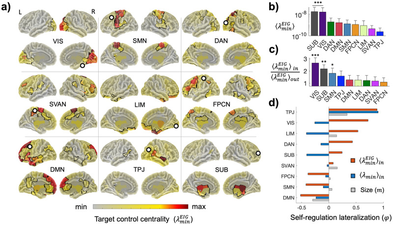
Identifying the driver nodes of a network has crucial implications in biological systems from unveiling causal interactions to informing effective intervention strategies. Despite recent advances in network control theory, results remain inaccurate as the number of drivers becomes too small compared to the network size, thus limiting the concrete usability in many real-life applications. To overcome this issue, we introduced a framework that integrates principles from spectral graph theory and output controllability to project the network state into a smaller topological space formed by the Laplacian network structure. Through extensive simulations on synthetic and real networks, we showed that a relatively low number of projected components can significantly improve the control accuracy. By introducing a new low-dimensional controllability metric we experimentally validated our method on N = 6134 human connectomes obtained from the UK-biobank cohort. Results revealed previously unappreciated influential brain regions, enabled to draw directed maps between differently specialized cerebral systems, and yielded new insights into hemispheric lateralization. Taken together, our results offered a theoretically grounded solution to deal with network controllability and provided insights into the causal interactions of the human brain.

Fig 1. Principles of low-dimensional network controllability.

a) Toy network with n = 7 nodes. Its state x = [x₁,x₂,…,x₇] can be seen as a signal over a graph. By exploiting the Laplacian eigenvectors V = [V₁,V₂,…,V₇] of the network, the signal x can be embedded in a spectral space via the graph Fourier transform (GFT) $\stackrel{\mathrm{~}}{x}=V^{T}x$. The resulting eigenstate $\stackrel{\mathrm{~}}{x}$ measures how the signal is spatially distributed across different topological scales, from coarser (${\stackrel{\mathrm{~}}{x}}_1,{\tilde{x}}_2,\dots$) to finer-grained ($\dots ,{\stackrel{\mathrm{~}}{x}}_{6,}{\stackrel{\mathrm{~}}{x}}_7$) ones. We can also define the inverse operation iGFT $x=V\stackrel{\mathrm{~}}{x}$ that is illustrated in this panel. b) Low-dimensional controllability in terms of linear-time invariant (LTI) network output control. Instead of focusing on the network state, the goal is to determine the input signal u(t) that steers a low-dimensional output given by the subset of the eigenstate $y\left(t\right)=H_r\tilde{x}\left(t\right){=C}^{EIG}x\left(t\right)$, where the output matrix C^EIG = H_rV^T is obtained by selecting and reordering a number r < n of spectral components via a filtering matrix H_r. In this example, the network has n = 7 nodes and the first r = 3 spectral components are selected and reordered arbitrarily. Here, the filtering matrix H_r is a 3×7 matrix whose elements are {h_1,2} = {h_2,1} = {h_3,7} = 1 and zero elsewhere.

Fig 2. Fundamental advantage of low-dimensional controllability.

a) Laplacian eigenvectors (or eigenmaps) for one realization of the hierarchical modular small-world network (HSWM). Colors identify the different spatial contributions of the nodes at increasingly finer topological scales. b) Control accuracy in terms of precision (δ) as a function of the number of eigenmaps. Different lines correspond to different number of drivers. Candidate drivers are progressively added according to their betweenness centrality values in a descending order. Results correspond to the mean values obtained from 100 simulated networks. c) Average node precision $⟨\delta ⟩=\frac{1}{n}{\sum }_{i=1}^n{\delta }_i$ (black) and representativeness$⟨\eta ⟩=\frac{1}{n}{\sum }_{i=1}^n{\eta }_i$ (grey) for single-driver control as a function of the number of eigenmaps. Dashed curves correspond to the total accuracy⟨δ⟩+⟨η⟩. Results correspond to the mean values obtained from 100 simulated networks. d) Schematic representation of a hierarchical modular small-world network (HSWM) whose target set is progressively expanded by including an increasing number of nodes m. The inclusion criterion starts with the nodes in one module and then continues by considering the nodes in the subsequent modules until the covering of the entire network. e) Average node total control accuracy ⟨δ⟩+⟨η⟩ for single-drivers as a function of the target size m. Magenta/green curves correspond to results obtained by averaging the total accuracy for the drivers inside/outside the target. Results correspond to the mean values obtained from 100 simulated networks.

Fig 3. Application to actual brain network functional states.

a) Power spectrum for the left somatomotor area contralateral to the imagined movement. Blue = motor imagery, red = resting state. Solid lines = average across blocks, shaded bands = standard deviation. The vertical dashed line spots out the values at 10 Hz extracted for all the regions of interest (ROIs=nodes) and used for the controllability analysis. b) Spatial distribution of the trial-averaged power spectrum at 10 Hz for the initial resting state and the final motor imagery state. The brain, viewed from above, frontal lobe upside, is obtained from the real MRI of the subject. Power spectrum density (PSD) values are here reported in decibel and show the typical motor-related power decrease occurring in the left somatomotor regions contralateral to the right-hand movement. For the controllability analysis, PSD values have been normalized so that μ₀ = 0, σ₀ = 9.27 for the resting state and μ_f = −5.33, σ_f = 4.59 for the motor imagery state. c) Connectivity matrix of the structural connectome obtained from the DTI data of the subject. The top-left block corresponds to the left hemisphere, while the bottom-right block corresponds to the right hemisphere. The links weights measure the number of axonal fascicles between ROIs and are reported in logarithmic scale for the sake of readability. The driver node, selected according to the highest between centrality, is the somatomotor area in the right hemisphere. d) Block-averaged control precision and representativeness for the real brain network data as function of the number of eigenmaps. The target is the entire network, i.e. m = n = 200. Input control signals are obtained solving Eq 3 using the parameters t_f = 1, dτ = 0.01, and ρ = 0.0043, 0.0121, 0.0234 respectively for one, eight and 64 drivers. Vertical bars denote standard deviations.

Fig 4. Single-driver controllability of brain networks.

a) The Yeo2011 brain atlas parcellation. Each of the 214 regions of interests (ROIs) are organized in 9 functional systems: the visual network VIS, the somatomotor network SMN, the dorsal attention network DAN, the saliency and ventral attention network SVAN, the limbic network LIM, the frontoparietal control network FPCN, the default mode network DMN, the temporoparietal junction TPJ, and the subcortical network SUB. b) Low-dimensional worst-case control centrality ${\lambda }_{min}^{EIG}$ values as a function of the number of eigenmaps r. Each point corresponds to a different node (ROI) controlling the entire brain. Colors code for different systems. Values are shown for a representative subject. By decreasing r all ${\lambda }_{min}^{EIG}$ values become positive and numerically reliable after a critical threshold r*. The inset illustrates the distribution of r* from all subjects (N = 6134). Note that the standard metric λ_min (r = n = 214) gives the lowest negative values making it difficult to interpret. c) Group-averaged spatial distribution of standard (|λ_min|) and low-dimensional (${\lambda }_{min}^{EIG}$) control centrality. Low-dimensional control centrality exhibits a significant reorganization compared to standard control centrality. The third row shows the ROIs that significantly gain (filled circles) or lose (empty circles) importance as compared to standard control (Sign test p≪ 10⁻⁶, Cohen’ |d|>0.5, S2 File).

Fig 5. Target controllability of brain systems.

a) Spatial distribution of group-averaged control centrality ${\lambda }_{min}^{EIG}$ when targeting each separate brain system. Target systems are contoured by black curves. Best drivers tend to fall within each target as indicated by the colorbar. White circles identify the best drivers outside the target (Tab 1). For each system results are illustrated for left (L) and right (R) hemisphere in both ventral (up) and dorsal (bottom) views. b) System controllability $〈{\lambda }_{min}^{EIG}〉$ as the mean control centrality of all the nodes targeting a specific system. Bars indicate group-averaged values and error bars standard deviations. Asterisks denote the systems whose controllability is significantly higher according to a post-hoc ANOVA analysis (p ≪ 10⁻⁶). The more the asterisks, the stronger the difference. Tukey-HSD Post-hoc ***p ≪ 10⁻⁶, **p < 0.001,*p < 0.05 (S2 File). c) Ratio between self-regulation ${〈{\lambda }_{min}^{EIG}〉}_{in}$ and external regulation ${〈{\lambda }_{min}^{EIG}〉}_{out}$ measured respectively by the mean control centrality of the nodes inside and outside a specific targeted system. Bars indicate group-averaged values and error bars standard deviations. Values have been log-transformed for the sake of readability. Asterisks denote the systems whose controllability ratio is significantly higher according to a post-hoc ANOVA analysis (p ≪ 10⁻⁶). The more the asterisks, the stronger the difference. Tukey-HSD Post-hoc ***p ≪ 10⁻⁶, **p < 0.001,* p < 0.05 (S2 File). d) System lateralization in termsof self-regulation from the right (R) and left (L) hemisphere $\phi =\frac{{\zeta }^R-{\zeta }^L}{{\zeta }^R+{\zeta }^L}$. Red colors correspond to low-dimensional controllability $\zeta ={〈{\lambda }_{min}^{EIG}〉}_{in}$.Blue colors correspond to standard controllability $={〈{\lambda }_{min}〉}_{in}$. Grey colors show the lateralization in terms of number of nodes of the systems in each hemisphere. Bars indicate group-averaged values and errorbars standard error means. Lateralization of low-dim. self-regulation significantly depends on the brain system (ANOVA, p ≪ 10⁻⁶).

Fig 6. Control relationships between brain systems.

a) The group-averaged controllability meta-graph. Nodes correspond to different brain systems. Directed weighted links illustrate the group-averaged geometric mean of the control centrality for system i when targeting system j ${〈{\lambda }_{min}^{EIG}〉}_{i\to j}$. The darker and thicker the link, the stronger the influence of system i on j. Self-loops and the SUB network are not represented as their control centrality is several orders of magnitudes higher. b) System control unbalance as the difference between the sum of outgoing and incoming weighted links from the individual meta-graphs. Positive values = tendency to act as driver. Negative value = tendency to act as target. Bars indicate group-averaged values and errorbars standard deviations. +/- denote the systems whose controllability is significantly higher/lower according to a post-hoc ANOVA analysis (p ≪ 10⁻⁶). The more the symbols, the stronger the differences. Tukey-HSD Post-hoc ***p ≪ 10⁻⁶, **p < 0.001 (S2 File). c) Hemispheric preference in terms of ipsilateral and contralateral control capacity. Dark colors denote ipsilateral control as the mean of the nodes in hemisphere i targeting the same hemisphere ${〈{\lambda }_{min}^{EIG}〉}_{i\to i}$. Light colors indicate contralateral control as the mean of the nodes in hemisphere i targeting the other hemisphere ${〈{\lambda }_{min}^{EIG}〉}_{i\to j}$. Bars indicate group-averaged values and errorbars standard deviations. L = left hemisphere, R = right hemisphere. Asterisks indicate Cohen’s d values measuring effect sizes. Sign test **p ≪ 10⁻⁶,Cohen’ |d|>0.5, *p ≪ 10⁻⁶, Cohen’ |d|>0.2, S2 File). d) Hemispheric preference of single systems in terms of their ability to control the entire ipsilateral and contralateral hemisphere. Same graphical conventions as before.

References

1. Liu YY, Barabási AL. Control Principles of Complex Networks. Rev Mod Phys [Internet]. 2016. Sep 6 [cited 2017 May 16];88(3). Available from: http://arxiv.org/abs/1508.05384
1. Gu S, Pasqualetti F, Cieslak M, Telesford QK, Yu AB, Kahn AE, et al. Controllability of structural brain networks. Nat Commun. 2015;6:8414. doi: 10.1038/ncomms9414 - DOI - PMC - PubMed
1. Liu YY, Slotine JJ, Barabási AL. Controllability of complex networks. Nature. 2011. May 12;473(7346):167–73. doi: 10.1038/nature10011 - DOI - PubMed
1. Jalili M, Askari Sichani O, Yu X. Optimal pinning controllability of complex networks: Dependence on network structure. Phys Rev E. 2015. Jan 5;91(1):012803. doi: 10.1103/PhysRevE.91.012803 - DOI - PubMed
1. Pasqualetti F, Zampieri S, Bullo F. Controllability Metrics, Limitations and Algorithms for Complex Networks. IEEE Trans Control Netw Syst. 2014. Mar;1(1):40–52.
LinkOut - more resources