. 2025 Jan 8;12(1):240763.
doi: 10.1098/rsos.240763. eCollection 2025 Jan.

Predicting the effect of landscape structure on epidemic invasion using an analytical estimate for infection rate

Affiliations

Predicting the effect of landscape structure on epidemic invasion using an analytical estimate for infection rate

Yevhen F Suprunenko et al. R Soc Open Sci. .

Abstract

The influence of landscape structure on epidemic invasion of agricultural crops is often underestimated in the construction and analysis of epidemiological models. Computer simulations of individual-based models (IBMs) are widely used to characterize disease spread under different management scenarios but can be slow in exploring large numbers of different landscape configurations. Here, we address the problem of finding an analytical measure of the impact of the spatial structure of a crop landscape on the invasion and spread of plant pathogens. We explore the potential of using an analytical approximation for the rate, r , at which susceptible crop fields become infected at the start of an epidemic to predict the effect that the spatial structure of a host landscape will have on an epidemic. We demonstrate the validity of this approach using two models: (i) a general IBM of the invasion and spread of a pathogen through an abstract host landscape; and (ii) an IBM of a real-life example for a virus disease spreading through a cassava landscape. Finally, we demonstrate that the analytical approach based on an estimate of the rate, r , can be used to identify spatial structures that effect deceleration of an invading pathogen.

Keywords: analytical approximation; crop landscape; epidemic invasion; epidemiological model; infection rate; spatially explicit individual-based model.


Conflict of interest statement

We declare we have no competing interests.

Figures
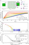
Effect of landscape configuration on epidemic progress in an agricultural crop landscape.
Figure 1.
Effect of landscape configuration on epidemic progress in an agricultural crop landscape. (a) Two examples of different spatial configurations described by the number of identical clusters Nclusters of the crop area (green) consisting of identical square fields (a field is an individual host unit in the IBM 1). The total crop area in all cases here represents 15% of the total area of a landscape. (b) Within the IBM 1, the probability that a susceptible individual field (green) is infected from an infected field (magenta) depends upon the product of a transmission rate and a dispersal kernel, βbx, for the pathogen. (c) Dynamics of the expected number of infected fields I(t) obtained from computer simulations of the IBM 1. (d) Values of I(t), shown as points, at an arbitrarily selected time, t=1.3 after invasion, in the interval between t=0.5 and t=1.5 where trajectories are well separated and can be easily distinguished visually; the intervals between 2.5% and 97.5% percentiles (shown as vertical bars) in the distribution of the number of infected fields in individual simulations. (e) Infection rate of susceptible fields becoming infected at the start of an epidemic estimated from simulations according to equation (2.1) using I0=1 and δt=0.1. Data and codes for all figures in this article are available from Figshare [34,35].
Performance of the analytical approximation for epidemic infection rate in IBM
Figure 2.
Performance of the analytical approximation for epidemic infection rate in IBM (equation 2.7), for different parameter values. (a) Parameters used in the IBM. The following values were considered: σ=1 km and 10 km; A0=0.2 km and 1 km; Nclusters varying from 1 until approximately 200×200;AH from 1% to 60% of A, where A is fixed as 365×365 km2. (b–d) Analytical estimates (solid lines) were compared with estimates from computer simulations (symbols) for different spatial scales of pathogen dispersal σ and landscapes. The infection rate is estimated from results of computer simulations in the same way as in figure 1e. Note, according to equation (2.7), the maximal value of r at Nclusters=1 is close to the value rmax=βnmax, where nmax1/A0, therefore rmax=25 in panels (b) and (d), and rmax=1 in panel (c). Results on the panel (c) for each value of AH/A separately are shown in electronic supplementary material, supplementary note S5.
A default (original) cassava landscape and two reconfigurations in Model 2.
Figure 3.
A default (original) cassava landscape and two reconfigurations in Model 2. (a) A sample area of the original rasterized cassava landscape map provided by Szyniszewska et al. [36] and converted to fields [24] (§2). (b) A sample area of the original landscape, denoted H, and its spatial re-configurations, denoted A and B; all three configurations are at 1 km resolution. Dashed and solid rectangles show 24 km-by-24 km and 8 km-by-8 km areas, respectively, that are used to estimate the infection rate analytically. The primary infected field is located at the intersection of solid black lines shown in landscape H in panel (b).
Computer simulations of an IBM of invasion and spread of CBSV through a default (original)
Figure 4.
Computer simulations of an IBM of invasion and spread of CBSV through a default (original) cassava landscape and two reconfigurations (Model 2 defined in §2). (a) Parameters of pathogen dispersal kernels b(x) sampled from posterior distribution of parameters p, α and β (modified from figure 3 in Godding et al. [24]). (be) Each column shows the dispersal kernel, corresponding results of computer simulations, and the estimates of infection rate calculated from simulations, and from equation (2.7) using 24 km-by-24 km area (denoted by r with a dashed rectangle as a subscript) and 8 km-by-8 km area (denoted by r with a solid rectangle as a subscript); these areas are shown in figure 3b. Estimates of infection rate from equation 2.7) were used to calculate the number of infected fields, exp(r×Δt), assuming exponential growth for Δt=1/12 year and compared with the mean value IΔt estimated from simulations. The median, 5% and 95% percentiles for 1000 individual simulations related to IΔt are shown in electronic supplementary material, figures S5 and S6, supplementary note S7.
Computer simulations of an IBM of invasion and spread of CBSV through a default
Figure 5.
Computer simulations of an IBM of invasion and spread of CBSV through a default (original) cassava landscape and two reconfigurations (Model 2 defined in §2), part 2. Same as figure 4 but using dispersal kernels with fixed parameters α and β and different values of the parameter p defined in (a). (a) Parameters of pathogen dispersal kernels b(x). (b–e) Dispersal kernels, results of computer simulations and estimates of the infection rate calculated from simulations and equation (2.7). Note, the dispersal kernel in panel (b) corresponds to the dispersal kernel in figure 4d.
Illustration of use of analytical approximation to inform local reconfiguring of host landscape to reduce epidemic spread.
Figure 6.
Illustration of use of analytical approximation to inform local reconfiguring of host landscape to reduce epidemic spread. (a) Pathogen dispersal kernel that corresponds to figure 4c. (b) Assuming that only a small fraction (approximately 3.5%, see text) of the host landscape can be reconfigured using type B, homogenization, we identified the preferred locations for local homogenization and constructed the corresponding landscape, denoted as Bpartial. The same sample area from three landscapes: the original (unmodified) landscape H, the partially homogenized landscape Bpartial where the locally homogenized areas are outlined by the red boundary and the fully homogenized landscape B. Two different initial locations of a primary infection are denoted as x1 and x2 and shown in landscape H. (c,d) Results of computer simulations of Model 2 using the dispersal kernel (a), the three landscapes (H, Bpartial and B) and two different primary locations of infection, x1 and x2. Here, the effect from type B reconfiguration is similar to the effect from increasing number of clusters Nclusters in figure 1: in both cases, the infection rates are reduced. Results for landscapes Bpartial and B appear nearly indistinguishable in both cases.

Similar articles

Cited by

References

    1. Meyfroidt P, et al. . 2022. Ten facts about land systems for sustainability. Proc. Natl Acad. Sci. USA 119, e2109217118. (10.1073/pnas.2109217118) - DOI - PMC - PubMed
    1. Phalan B, Onial M, Balmford A, Green RE. 2011. Reconciling food production and biodiversity conservation: land sharing and land sparing compared. Science 333, 1289–1291. (10.1126/science.1208742) - DOI - PubMed
    1. Grass I, et al. . 2019. Land‐sharing/‐sparing connectivity landscapes for ecosystem services and biodiversity conservation. People Nat. 1, 262–272. (10.1002/pan3.21) - DOI
    1. Segre H, Carmel Y, Shwartz A. 2022. Economic and not ecological variables shape the sparing–sharing trade‐off in a mixed cropping landscape. J. Appl. Ecol. 59, 779–790. (10.1111/1365-2664.14092) - DOI
    1. Correa Ayram CA, Mendoza ME, Etter A, Salicrup DRP. 2016. Habitat connectivity in biodiversity conservation. Prog. Phys. Geogr. 40, 7–37. (10.1177/0309133315598713) - DOI

LinkOut - more resources