Estimating the Exposure-Response Relationship between Fine Mineral Dust Concentration and Coccidioidomycosis Incidence Using Speciated Particulate Matter Data: A Longitudinal Surveillance Study

Abstract

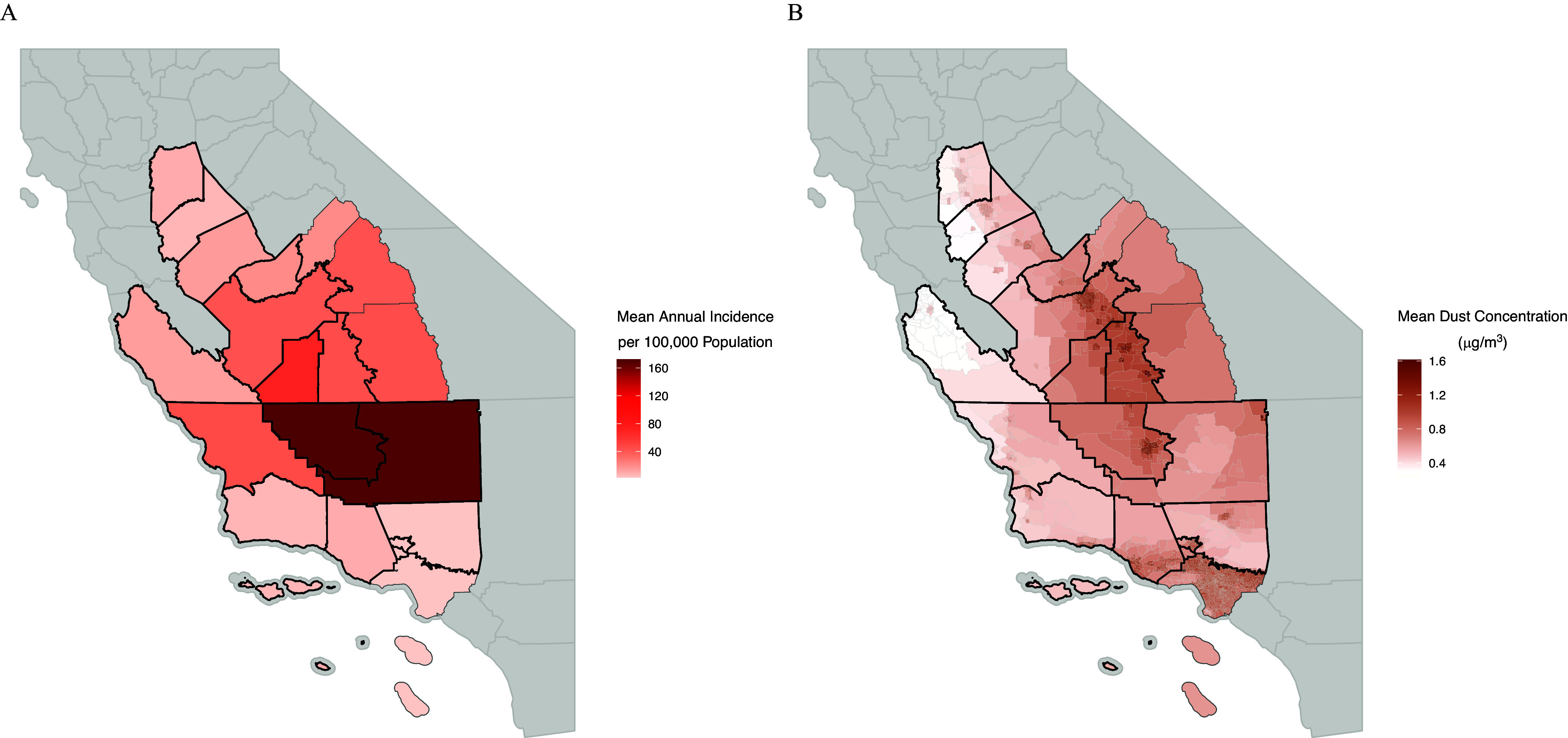
Background: Coccidioidomycosis, caused by inhalation of Coccidioides spp. spores, is an emerging infectious disease that is increasing in incidence throughout the southwestern US. The pathogen is soil-dwelling, and spore dispersal and human exposure are thought to co-occur with airborne mineral dust exposures, yet fundamental exposure-response relationships have not been conclusively estimated.

Objectives: We estimated associations between fine mineral dust concentration and coccidioidomycosis incidence in California from 2000 to 2017 at the census tract level, spatiotemporal heterogeneity in exposure-response, and effect modification by antecedent climate conditions.

Methods: We acquired monthly census tract-level coccidioidomycosis incidence data and modeled fine mineral dust concentrations from 2000 to 2017. We fitted zero-inflated distributed-lag nonlinear models to estimate overall exposure-lag-response relationships and identified factors contributing to heterogeneity in exposure-responses. Using a random-effects meta-analysis approach, we estimated county-specific and pooled exposure-responses for cumulative exposures.

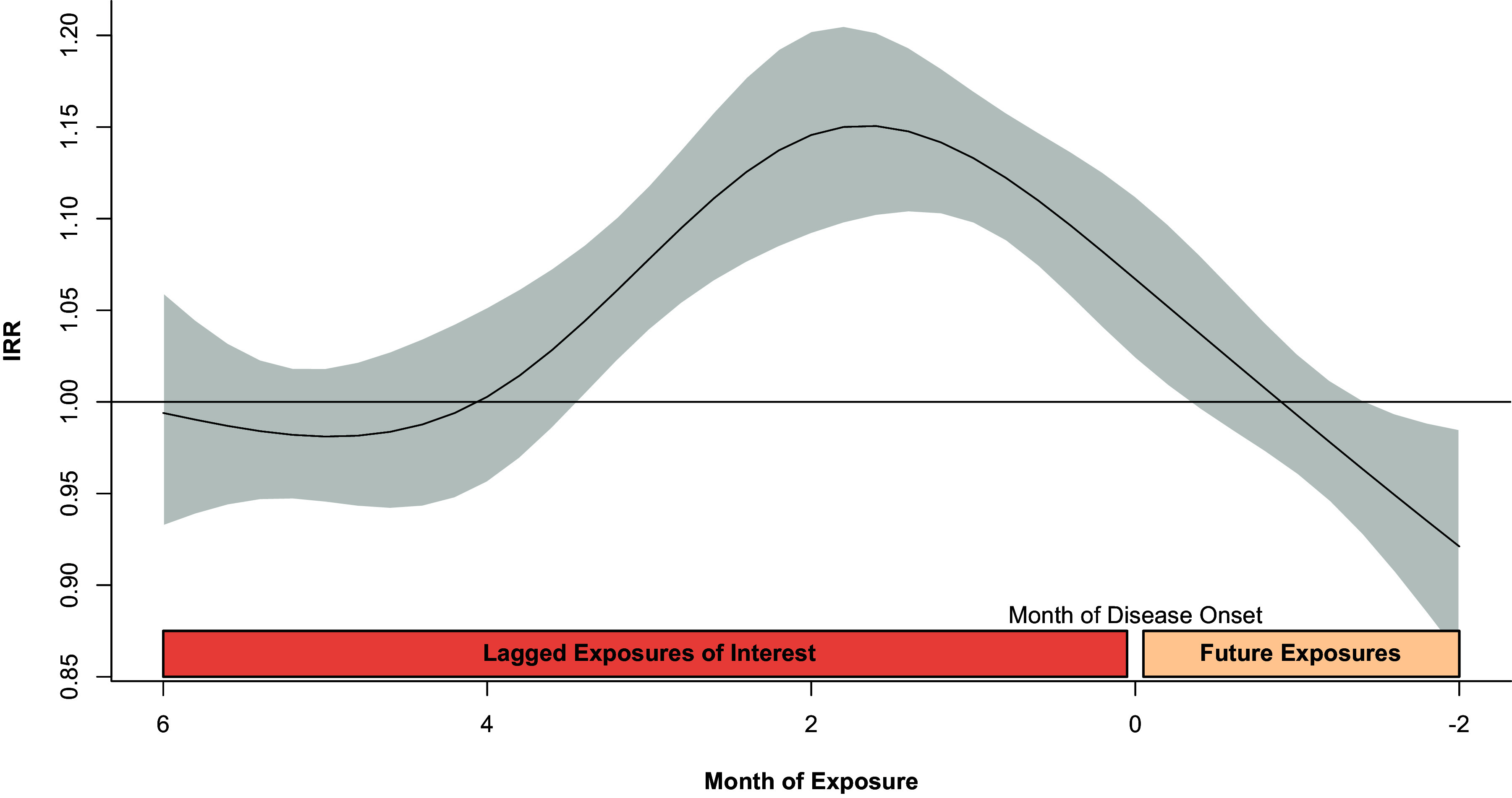
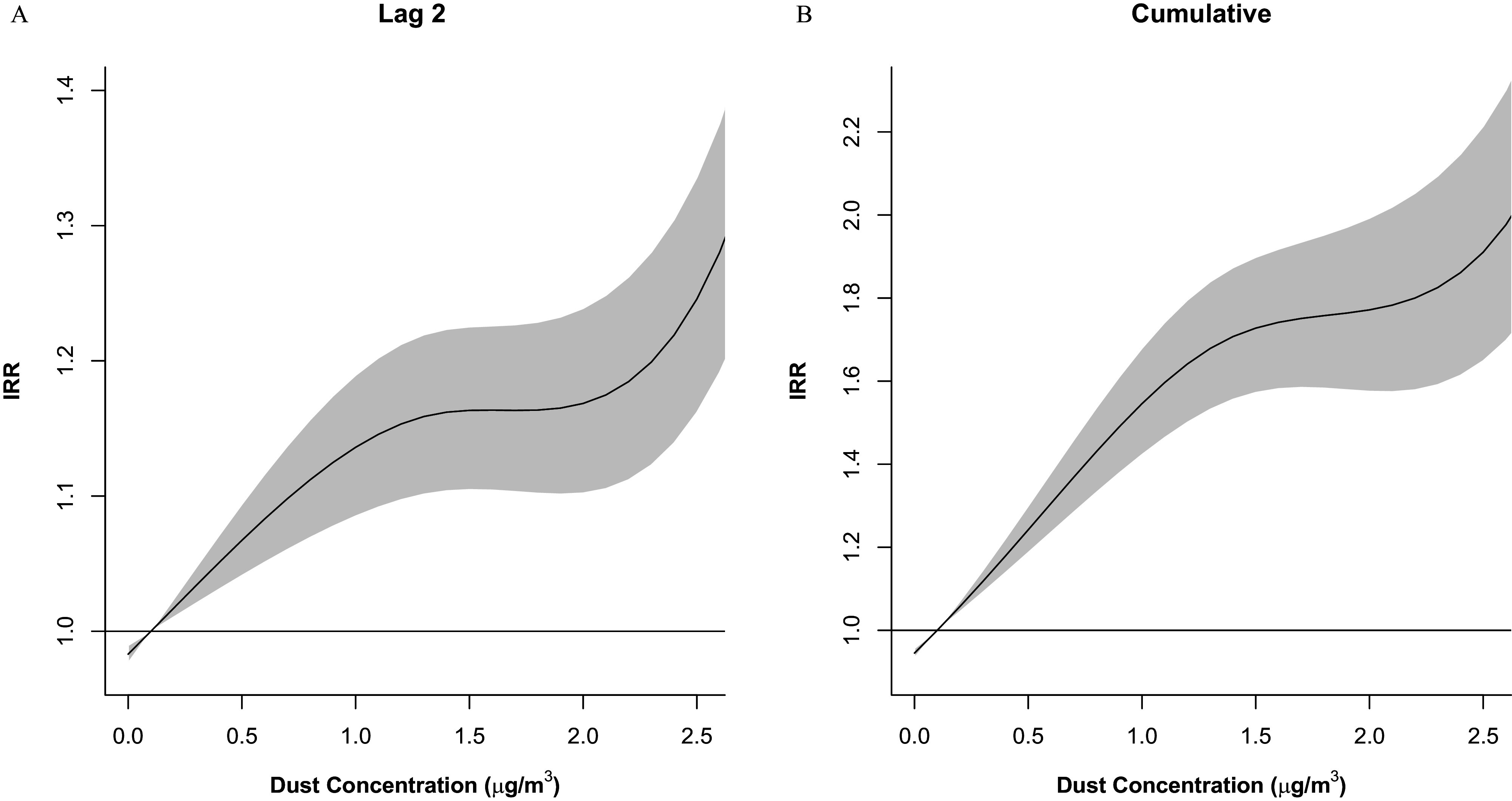
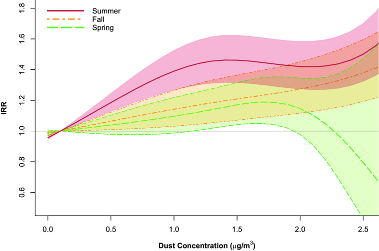
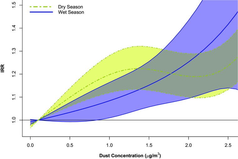
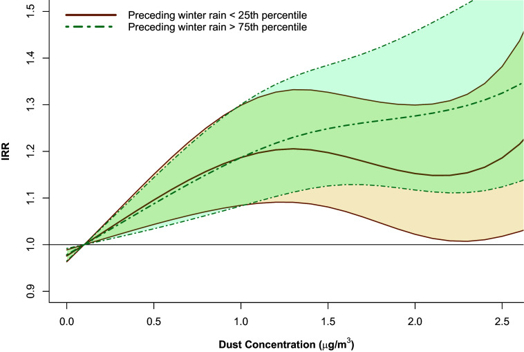
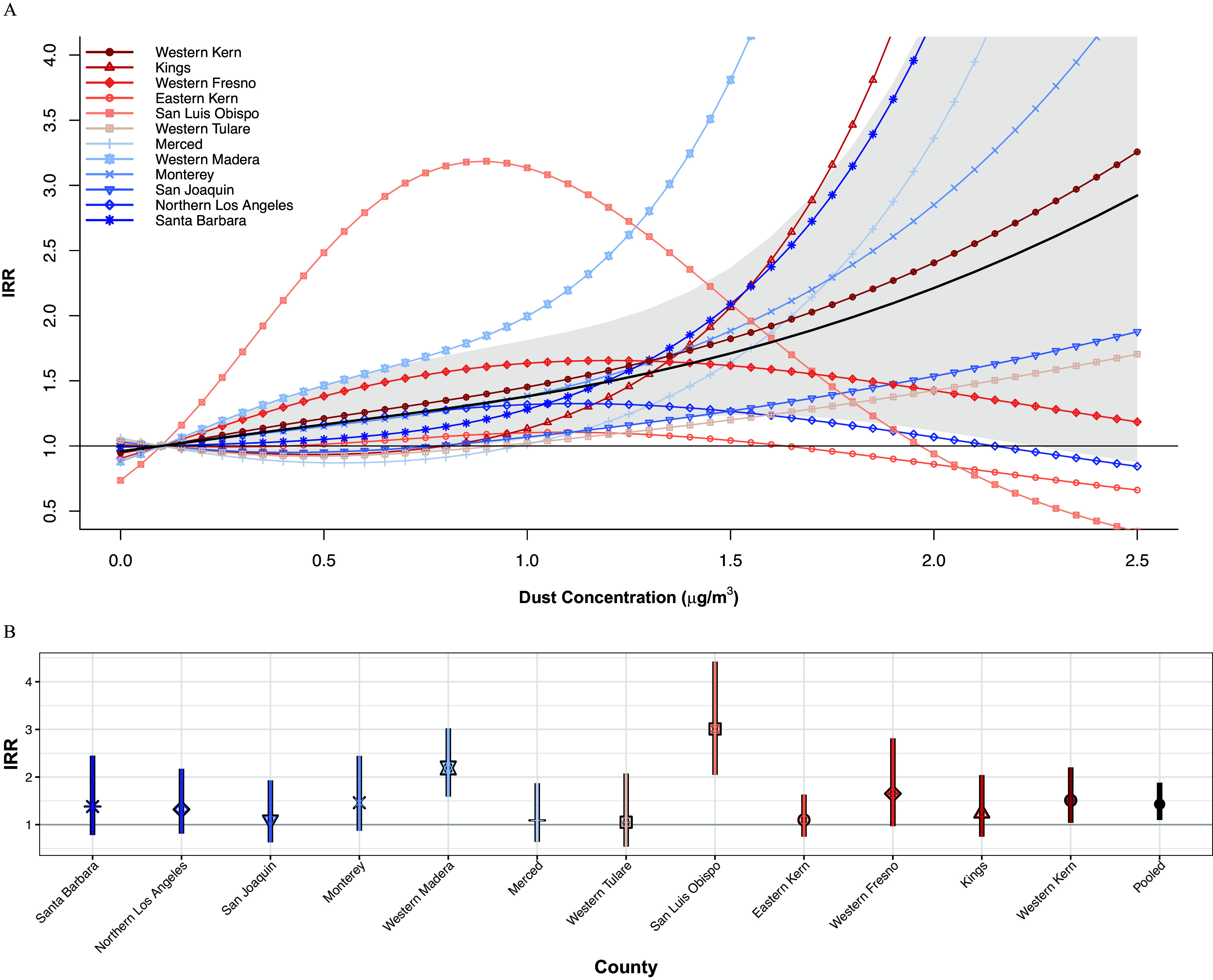
Results: We found a positive exposure-response relationship between cumulative fine mineral dust exposure in the 1-3 months before estimated disease onset and coccidioidomycosis incidence across the study region [incidence rate ratio (IRR) for an increase from 0.1 to $1.1{\mu g/m}^3=1.60$; 95% CI: 1.46, 1.74]. Positive, supralinear associations were observed between incidence and modeled fine mineral dust exposures 1 [$\text{IRR}=1.13$ (95% CI: 1.10, 1.17)], 2 [$\text{IRR}=1.15$ (95% CI: 1.09, 1.20)] and 3 [$\text{IRR}=1.08$ (95% CI: 1.04, 1.12)] months before estimated disease onset, with the highest exposures being particularly associated. The cumulative exposure-response relationship varied significantly by county [lowest IRR, western Tulare: 1.05 (95% CI: 0.54, 2.07); highest IRR, San Luis Obispo: 3.01 (95% CI: 2.05, 4.42)]. Season of exposure and prior wet winter were modest effect modifiers.

Discussion: Lagged exposures to fine mineral dust were strongly associated with coccidioidomycosis incidence in the endemic regions of California from 2000 to 2017. https://doi.org/10.1289/EHP13875.

Figure 1.

Maps of the study region, highlighting coccidioidomycosis incidence and fine mineral dust concentration over the study period (2000–2017) in California. The thick black outline denotes the included counties and subcounties in the study region ($N\text{\hspace{0.17em}counties}=14$; $N\text{\hspace{0.17em}census tracts}=515$). Census tracts and county subregions outside of the thickest black lines were not included in the analysis. (A) Full counties colored by their mean annual incidence of coccidioidomycosis per 100,000 population over the study period (2000 to 2017). Incidence is calculated at the county level as opposed to the subcounty level in accordance with CDPH policy. (B) Average monthly fine mineral dust concentrations (${\mathrm{\mu }\text{g}/\mathrm{m}}^3$) across the study region and period at the census tract level. Corresponding numerical data are shown in Excel Table S1. Note: CDPH, California Department of Public Health.

Figure 2.

Overall lag–response relationship for a 0.1- to $1.1\text{-}{\mathrm{\mu }\mathrm{g}/\mathrm{m}}^3$ increase in fine mineral dust concentration ($N\text{\hspace{0.17em}observations}=\mathrm{105,564}$) from this time-series ecological study based in California (2000–2017). IRRs were obtained from the DLNM testing the association between fine mineral dust concentration and coccidioidomycosis incidence using Equation 1. All models were adjusted for spatiotemporal trends. The x-axis represents the lag or lead of exposure comparison, with the month of zero indicating the month of estimated disease onset. Negative months indicate future exposures, which are used as negative controls. The y-axis represents the associated IRR. The solid line represents point estimates, and shading represents the 95% confidence interval. Corresponding numerical data are shown in Excel Table S2. Note: DLNM, distributed-lag nonlinear model; IRR, incidence rate ratio.

Figure 3.

Exposure–response relationships comparing $0.1{\mathrm{\mu }\mathrm{g}/\mathrm{m}}^3$ to a range of dust concentration values ($N\text{\hspace{0.17em}observations}=\mathrm{105,564}$) from this time-series ecological study based in California (2000–2017). IRRs estimated from the DLNM using Equation 1. All models were adjusted for spatiotemporal trends. The x-axis (fine mineral dust concentration) ranges from $0{\mathrm{\mu }\mathrm{g}/\mathrm{m}}^3$ to the 99th percentile of dust concentrations across the region ($2.52{\mathrm{\mu }\mathrm{g}/\mathrm{m}}^3$). The y-axis represents the associated IRR. (A) Exposure–response for lag 2 months. (B) Cumulative exposure–response over lag 1 to lag 3 months before disease onset. The solid line represents point estimates, and shading represents the 95% confidence interval. Corresponding numerical data are shown in Excel Table S3. Note: DLNM, distributed-lag nonlinear model; IRR, incidence rate ratio.

Figure 4.

Exposure–response relationship for increasing dust concentration at lag 2 months prior to estimated disease onset by season of dust exposure using DLNM Equation 3 ($N\text{\hspace{0.17em}observations}=\mathrm{105,564}$) from this time-series ecological study based in California (2000–2017). All models were adjusted for spatiotemporal trends. The x-axis (fine mineral dust concentration) ranges from $0{\mathrm{\mu }\mathrm{g}/\mathrm{m}}^3$ to the 99th percentile of dust concentrations across the region ($2.52{\mathrm{\mu }\mathrm{g}/\mathrm{m}}^3$). The y-axis represents the associated IRR. The months of March–May were coded as spring, June–August as summer, September–November as fall, and December–February as winter. Center lines are patterned by season of exposure and represent point estimates. The shading represents the 95% confidence interval. Corresponding numerical data are shown in Excel Table S4. Note: DLNM, distributed-lag nonlinear model; IRR, incidence rate ratio.

Figure 5.

Exposure–response relationship for increasing dust concentration at lag 2 months prior to estimated disease onset by precipitation season of dust exposure using DLNM Equation 4 ($N\text{\hspace{0.17em}observations}=\mathrm{105,564}$) from this time-series ecological study based in California (2000–2017). All models were adjusted for spatiotemporal trends. The x-axis (fine mineral dust concentration) ranges from $0{\mathrm{\mu }\mathrm{g}/\mathrm{m}}^3$ to the 99th percentile of dust concentrations across the region ($2.52{\mathrm{\mu }\mathrm{g}/\mathrm{m}}^3$). The y-axis represents the associated IRR. May–October was considered the dry season, and November–April the wet season. Center lines are patterned by season of exposure and represent point estimates. The shading represents the 95% confidence interval. Corresponding numerical data are shown in Excel Table S5. Note: DLNM, distributed-lag nonlinear model; IRR, incidence rate ratio.

Figure 6.

Exposure–response relationships comparing wet and dry winters as defined by exceeding the 75th percentile or falling below the 25th percentile of county-level winter precipitation using DLNM Equation 5 ($N\text{\hspace{0.17em}observations}=\mathrm{105,564}$) from this time-series ecological study based in California (2000–2017). All models were adjusted for spatiotemporal trends. The x-axis (fine mineral dust concentration) ranges from $0{\mathrm{\mu }\mathrm{g}/\mathrm{m}}^3$ to the 99th percentile of dust concentrations across the region ($2.52{\mathrm{\mu }\mathrm{g}/\mathrm{m}}^3$). The y-axis represents the associated IRR. Exposure–response curves are for increases in dust concentration at lagged 2 months prior to estimated disease onset. Center lines are patterned by winter precipitation category and represent point estimates. The shading represents the 95% confidence interval. Corresponding numerical data are shown in Excel Table S6. Note: DLNM, distributed-lag nonlinear model; IRR, incidence rate ratio.

Figure 7.

(A) County-specific best linear unbiased predictions and pooled region-wide estimate for cumulative dust exposures from 1 to 3 months prior to estimated disease onset using DLNM Equation 7 ($N\text{\hspace{0.17em}observations}=\mathrm{105,564}$) from this time-series ecological study based in California (2000–2017). All models were adjusted for spatiotemporal trends. The x-axis (fine mineral dust concentration) ranges from $0{\mathrm{\mu }\mathrm{g}/\mathrm{m}}^3$ to the 99th percentile of dust concentrations across the region ($2.52{\mathrm{\mu }\mathrm{g}/\mathrm{m}}^3$). The y-axis represents the associated IRR. Lines and symbols represent county-specific exposure–response relationships and are colored by subcounty annual incidence over the study period (i.e., including by eastern and western regions). Counties with high total cases during the study period are in red, and lower total cases in blue. The thick black line represents the pooled association. The solid lines represent point estimates, and shading represents the 95% confidence interval for the pooled estimate. (B) Point estimates and 95% confidence intervals for a 1-unit comparison centered at $0.1{\mathrm{\mu }\mathrm{g}/\mathrm{m}}^3$. Point estimates are colored according to subcounty annual incidence as in (A) and use the same symbol. Corresponding numerical data are shown in Excel Table S7. Note: DLNM, distributed-lag nonlinear model; IRR, incidence rate ratio.

References

1. Sondermeyer Cooksey GL, Nguyen A, Vugia D, Jain S. 2020. Regional analysis of coccidioidomycosis incidence—California, 2000–2018. MMWR Morb Mortal Wkly Rep 69(48):1817–1821, PMID: 33270616, 10.15585/mmwr.mm6948a4. - DOI - PMC - PubMed
1. Cox RA, Magee DM. 1998. Protective immunity in coccidioidomycosis: the life cycle and biology of Coccidioides immitis. Res Immunol 149(4–5):417–428, PMID: 9720959, 10.1016/s0923-2494(98)80765-7. - DOI - PubMed
1. Kirkland TN, Fierer J. 2018. Coccidioides immitis and posadasii; a review of their biology, genomics, pathogenesis, and host immunity. Virulence 9(1):1426–1435, PMID: 30179067, 10.1080/21505594.2018.1509667. - DOI - PMC - PubMed
1. Weaver E, Kolivras KN, Thomas RQ, Thomas VA, Abbas KM. 2020. Environmental factors affecting ecological niche of Coccidioides species and spatial dynamics of valley fever in the United States. Spat Spatiotemporal Epidemiol 32:100317, PMID: 32007282, 10.1016/j.sste.2019.100317. - DOI - PubMed
1. CDC (Centers for Disease Control and Prevention). n.d. Valley Fever. https://www.cdc.gov/fungal/diseases/coccidioidomycosis/index.html [accessed 1 May 2022].
LinkOut - more resources