Dynamical constraints on neural population activity

Abstract

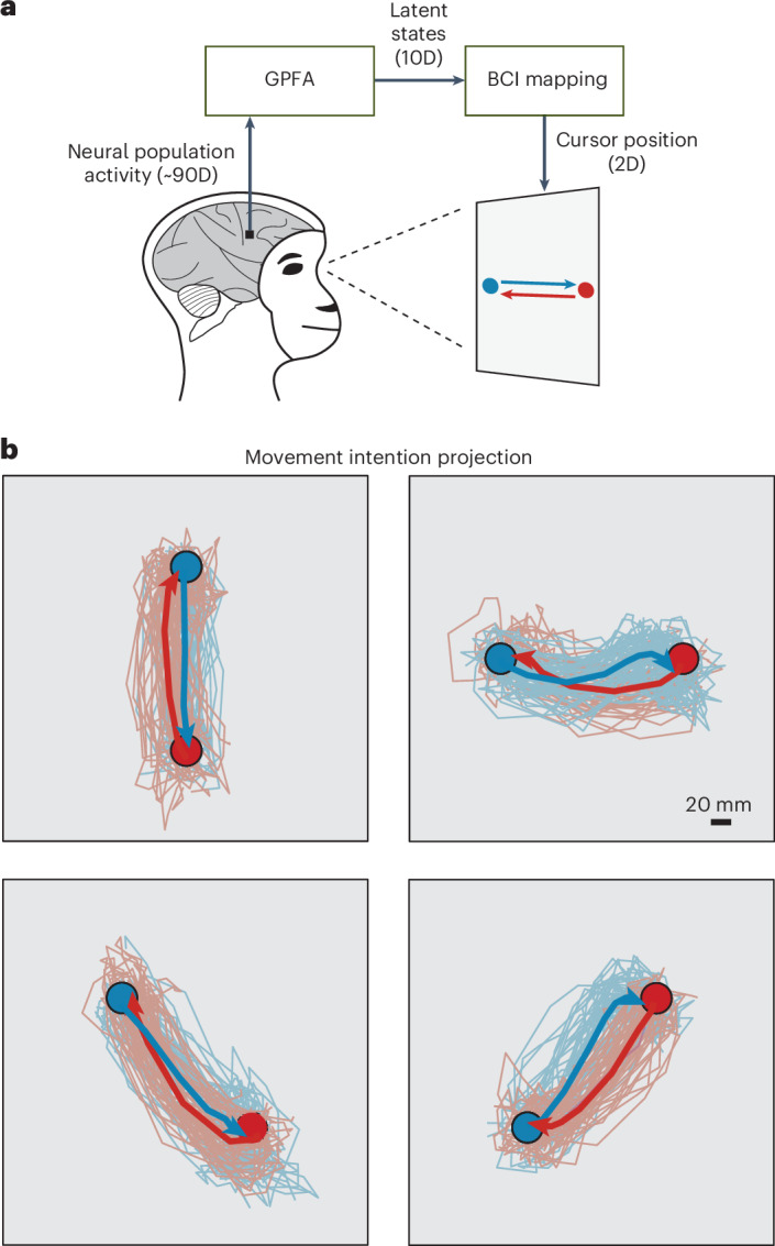
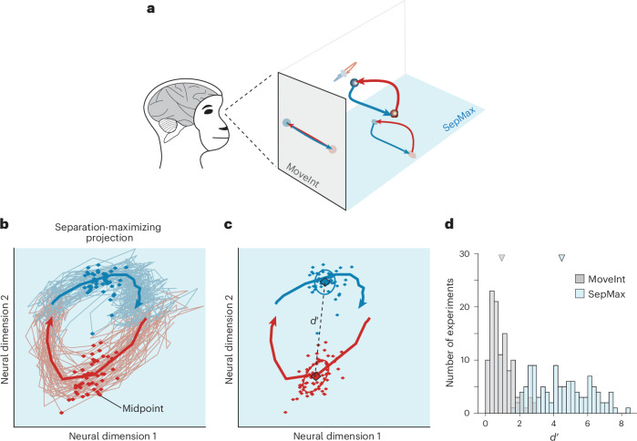
The manner in which neural activity unfolds over time is thought to be central to sensory, motor and cognitive functions in the brain. Network models have long posited that the brain's computations involve time courses of activity that are shaped by the underlying network. A prediction from this view is that the activity time courses should be difficult to violate. We leveraged a brain-computer interface to challenge monkeys to violate the naturally occurring time courses of neural population activity that we observed in the motor cortex. This included challenging animals to traverse the natural time course of neural activity in a time-reversed manner. Animals were unable to violate the natural time courses of neural activity when directly challenged to do so. These results provide empirical support for the view that activity time courses observed in the brain indeed reflect the underlying network-level computational mechanisms that they are believed to implement.

Fig. 1. Testing the flexibility of the time courses of neural population activity.

a, Activity recorded from a population of neurons is binned in time (for example, tens of milliseconds) and represented in a population activity space, where each axis represents the firing rate of one of the recorded neurons. The time course of the population activity patterns forms a neural trajectory (red line). For illustration purposes, a three-electrode recording is shown, corresponding to a three-dimensional population activity space. In our actual experiments, ~90 electrodes were used. b,c, The central question of this study is whether neural population activity patterns can be generated in different orderings. b, An example of a different ordering of the same population activity patterns that comprise the trajectory shown in a. In this example, the start and endpoints of the trajectory are the same as in a, but the activity patterns are produced in a different order. Although it appears that the trajectory intersects with itself, in the 3D population activity space it is not intersecting. c, A depiction of the time-reversal of the trajectory shown in a.

Fig. 2. Monkeys can move the BCI cursor in any direction in the MoveInt projection.

a, The BCI provides the monkey with moment-by-moment visual feedback of its population activity patterns as they evolve over time. We used a causal version of GPFA to estimate 10D latent states at each time step based on the recorded population activity (~90D). We then provided the monkey with visual feedback of two dimensions of its latent states (defined by a BCI mapping; Methods), which determine the moment-by-moment 2D position of the BCI cursor. The monkey moved the cursor from target A to target B (blue) and from target B to target A (red). b, Cursor trajectories for the four possible target pairs while using the MoveInt BCI mapping. For visualization, trajectories are colored by the start target (for example, red trajectories indicate movements originating at the red target and moving to the blue target). Thin traces represent individual trial trajectories. Thick traces represent trial-averaged trajectories. Note the high degree of overlap between the red trajectories and blue trajectories for each target pair.

Fig. 3. Neural trajectories follow direction-dependent paths in the 10D activity space.

a, The MoveInt mapping provides the monkey feedback of one particular 2D projection of the neural trajectories. In the MoveInt projection (indicated by the gray background), the A-to-B (blue) and B-to-A (red) trajectories overlap. However, when we examine the 10D space in which the neural trajectories reside, we find that the A-to-B (blue) trajectories are distinct from the B-to-A (red) trajectories. The SepMax projection is indicated by the light blue background. b, The SepMax projection is a 2D projection of the neural trajectories in which the A-to-B (blue) trajectories are distinct from the B-to-A (red) trajectories. Thin traces show trajectories for individual trials. Diamonds indicate the midpoint (Methods) for each trial. Thick traces represent trial-averaged trajectories. c, We quantify the separation between red and blue trajectories in 10D space as the discriminability (d′) of the blue and red midpoints. Computing d′ involves the separation of the means (dashed line) and the covariances (ellipses) of the trial-to-trial scatter (Methods). d, Across all experiments (n = 111), the neural trajectories are substantially more separated in the SepMax projection (d′ = 4.5 ± 1.6; mean ± s.d.) than they are in the MoveInt projection (d′ = 0.9 ± 0.6; mean ± s.d.; two-sided t test, P < 10⁻⁴¹). Means are indicated by the triangles.

Fig. 4. Direction-dependent paths of neural trajectories persist even when BCI feedback is given in the SepMax projection.

a,b, The BCI paradigm allows us to choose which 2D projection of the neural trajectories we provide the monkey as visual feedback. Rather than show the monkey the MoveInt projection (gray background) (a), we rotate the population activity space relative to the monitor to show him the SepMax projection (light blue background) (b). c, Under the SepMax projection, we tested if the direction-dependent paths observed during the MoveInt block would persist (possibility 1) or if the monkey would straighten out its cursor trajectories (possibility 2). d, Neural trajectories are similar whether the MoveInt or SepMax projection is used for feedback. When the monkey received visual feedback of the MoveInt projection (top row), the A-to-B trajectories (blue) overlapped with the B-to-A trajectories (red) in the MoveInt projection (top left; gray background). Black outline indicates the projection that provides the monkey with visual feedback on the monitor. Those same trajectories are distinct in the SepMax projection (top right; light blue background). When the monkey received visual feedback of the SepMax projection (bottom row), the trajectories continued to follow direction-dependent paths (bottom right; light blue background). Those same trajectories overlap in the MoveInt projection (bottom left; gray background). e, Same trials as shown in d (bottom right), separated into ‘early’ trials, that is, the first half (50 trials for this session, left), and ‘late’ trials, that is, the second half (49 trials for this session, right). f, We calculated d′ separately for the early trials and the late trials and computed $\mathrm{\Delta }{d}^{\prime }=d_{\mathrm{early}}^{\prime }-d_{\mathrm{late}}^{\prime }$ to determine whether the animal straightened out its trajectories. As a reference, we also calculated $\mathrm{\Delta }{d}^{\prime }$ for the same trajectories partitioned randomly into two groups. Across all experiments, the change in separation of ‘early’ versus ‘late’ trial trajectories ($\mathrm{\Delta }{d}^{\prime }$ = 0.07 ± 1.1, mean ± s.d.) was similar to that of the shuffle control ($\mathrm{\Delta }{d}^{\prime }$ = 0.01 ± 1.2, mean ± s.d.; two-sided t test, P = 0.69, n = 111). Means are indicated by the triangles. Example session indicated with circles.

Fig. 5. Neural trajectories are robust to which projection provides the visual feedback.

a, We used flow fields to compare activity time courses across conditions. We calculated a separate flow field for each target condition, that is, cursor movements from A to B (blue) and cursor movements from B to A (red), to capture how the neural trajectory unfolds from a given initial condition. The flow fields for each condition are plotted together to visualize the overall flow. Each panel corresponds to Fig. 4d. Length and direction of arrows indicate the average, observed cursor velocity as a function of position in the corresponding 2D space. Arrows are colored by the direction of the cursor movement, and the color saturation indicates the number of data points that contribute to the average. The flow fields in the SepMax projection when seen (black outline) and unseen (no outline) by the monkey were similar (comparison noted by the large light blue arrow). In contrast, the flow field in the SepMax projection differed from the flow field in the MoveInt projection (comparison noted by large black arrow). b, We quantified the similarities between the flow fields by calculating the mean squared difference of the corresponding flow field vectors (Methods). The flow fields in the SepMax projection were similar regardless of whether they were seen or unseen by the monkey (vertical axis, cf. large light blue arrow in a). For reference, we considered a case where the flow fields were different, namely for the two projections that we used to provide visual feedback to the monkey (horizontal axis, cf. large black arrow in a). Filled symbols indicate sessions where the flow field difference in the SepMax projection across the two feedback projections (vertical axis) was significantly smaller than the flow field difference between the different feedback projections (horizontal axis, two-sided Wilcoxon rank-sum, P < 0.05, 90 of 111 sessions—48 of 50 sessions for monkey E, 23 of 40 sessions for monkey D and 19 of 21 sessions for monkey Q. Paired t test P < 10⁻¹⁶, n = 111 sessions). Red dot indicates the example session shown in a.

Fig. 6. Challenging monkeys to violate the flow field.

a, Flow fields (small arrows) characterize the distinct paths (large arrows) as the monkey moves the cursor from A to B (blue) and B to A (red). b, We sought to assess if the monkey could produce a trajectory that moves against the flow field. c, To challenge the monkeys to move against the flow field, we placed an intermediate target (IT; black circle) along the path of the flow field. Black lines represent single-trial cursor trajectories (thin lines) and the trial-averaged cursor trajectory (thick line) to the IT. d, To quantify the animal’s ability to move the cursor against the flow field, we measured the initial angle between the trajectory to the IT (black line) relative to the direct path to the IT (dashed line). For comparison, we measured the initial angle between the cursor trajectory to the blue target in the two-target task (red line; cf. Fig. 4d) and the direct path to the IT. e, Distribution of the percentage difference of the two initial angles illustrated in d across experiments. A 0% difference (vertical dashed line, left) indicates that the cursor moves along the flow field before acquiring the IT. A 100% difference (vertical dashed line, right) indicates that the cursor was able to move straight to the IT (against the flow field). The percentage difference is not statistically different from zero (two-sided t test, P = 0.84, n = 50). f, For the ‘no change’ control, we compute the initial angles between the early (red line, same as in d) and late (dashed red line) two-target trials relative to the direct path to the IT (dashed black line). g, ‘No change’ distribution across experiments. This distribution is not statistically different from zero (two-sided t test, P = 0.61, n = 50). h, For the ‘full-change’ control, we show the first nine time points of trial-averaged center-out cursor trajectories under the MoveInt projection (cf. Fig. 2b). We measured the initial angle relative to the direct path to the cued target (dashed line for the example shown) for trajectories to the cued target compared to trajectories to the neighboring +45° and −45° targets. Here we highlight the initial angles for the blue trajectory (cued target) and the aqua trajectory (−45° target). i, ‘Full-change’ distribution across experiments. The distribution is statistically different from zero (two-sided t test, P < 10⁻²⁸, n = 50) and from 100% change (two-sided t test, P = 0.008, n = 50).

Fig. 7. Monkeys did not generate time-reversed neural trajectories.

a, The monkeys performed an ‘instructed path task’, in which they had to move the cursor from the start target (red circle) to the IT (black circle) without exiting a visual boundary (oval outline). b, To encourage the monkeys to modify their trajectories, we incrementally reduced the size of the boundary so that an inability to alter their trajectories would eventually lead to a failure at the task. Cursor trajectories for the least and most restrictive paths for an example session. The least restrictive path (left) minimally affected the cursor trajectories relative to the unconstrained trajectories (cf. Fig. 6c). With the most restrictive path, the animal only succeeded approximately half the time (right). Successful trials are shown as thin black lines. Failed trials are shown as thin red lines. The thick black line shows the average of all trials, regardless of success, for that boundary size. c, The five boundary sizes (oval outlines in different shades of gray; size refers to the distance of the boundary from the target indicated by the dashed line) and trial-averaged cursor trajectories of successful trials only for each boundary size (line in corresponding shade of gray) for the example session. d, Comparison of the initial angle of the most constrained trials (trial-averaged trajectory of all initiated trials regardless of eventual success, black line) to the initial angle of the two-target trials (trial-averaged trajectory of all initiated trials regardless of eventual success, red line; same as in Fig. 6d,f). We calculated the initial angles relative to the direct path (black dashed line) from the start target (red circle) to the IT (black circle). e, Distribution of the percentage difference in initial angle across experiments (n = 50). The mean is indicated by the black triangle. For reference, the no-change distribution (dark red triangle and line; mean ± s.d.) and the full-change distribution (gray triangle and line; mean ± s.d.) from Fig. 6 are shown here.

Extended Data Fig. 1. Results hold for each animal individually.

a–c, Per animal results for Fig. 3d. For each animal individually, the neural trajectories are substantially more separated in the SepMax projection than in the MoveInt projection. a, Monkey E. SepMax d′ = 5.6 ± 1.2 (mean ± s.d.), MoveInt d′ = 0.9 ± 0.6 (mean ± s.d.; two-sided t-test, p < 10⁻⁵, N = 50). b, Monkey D. SepMax d′ = 2.9 ± 0.9 (mean ± s.d.), MoveInt d′ = 1.1 ± 0.8 (mean ± s.d.; two-sided t-test, p < 10⁻³, N = 40). c, Monkey Q. SepMax d′ = 4.7 ± 1.2 (mean ± s.d.), MoveInt d′ = 0.7 ± 0.4 (mean ± s.d.; two-sided t-test, p = 0.0035, N = 21). d–f, Per animal results for Fig. 6e,g,i. Distribution of the percent difference of the two initial angles (black; monkey E: 2.4 ± 15.4%, monkey D: 0.29 ± 28.5%, monkey Q: −7.6 ± 20.4%, mean ± std) illustrated in Fig. 6d. Zero percent difference (vertical dashed line, left) indicates that the cursor moves along the flow field before acquiring the intermediate target. One hundred percent difference (vertical dashed line, right) indicates that the cursor was able to move straight to the intermediate target (that is, against the flow field). For reference, the no-change distribution (dark red triangle and line; monkey E: −11.3 ± 33.0%, monkey D: 4.5 ± 10.5%, monkey Q: 13.3 ± 16.7%; mean ± std) and the full-change distribution (gray triangle and gray line; monkey E: 88.6 ± 30.9%, monkey D: 93.7 ± 13.7% monkey Q: 87.9 ± 26.7%; mean ± std) are shown here, computed separately for each monkey. For monkeys E and D, the change in initial angle in the intermediate-target task is not statistically different from the ‘no change’ condition (two-sided t-test; monkey E: p = 0.06, N = 28; monkey D: p = 0.6, N = 9), but is statistically different from the ‘full-change’ condition (two-sided t-test; monkey E: p < 10⁻¹⁵, N = 28; monkey D: p < 10⁻⁵, N = 9). For Monkey Q, the change in initial angle in the intermediate-target task is less than the ‘no change’ condition (two-sided t-test, p = 0.03, N = 13) and is statistically different from the ‘full-change’ condition (two-sided t-test, p < 10⁻⁷, N = 13). g–i. Per animal results for Fig. 7e. Distribution of the percent difference of the two initial angles (black; monkey E: 9.4 ± 30.9%; monkey D: 19.0 ± 13.7%; monkey Q: 26.4 ± 26.7%, mean ± std) illustrated in Fig. 7d. Also shown is the distribution for the no change control (red) and the distribution for the full-change control (gray), computed separately for each monkey. There is a small change in the initial angle of the trajectories compared to the ‘no change’ condition (two-sided t-test; monkey E: p = 10⁻³, N = 28; monkey D: p = 0.09, N = 9; monkey Q: p = 0.01, N = 13), but did not approach the ‘full-change’ condition (two-sided t-test; monkey E: p < 10⁻¹¹, N = 28; monkey D: p < 10⁻⁴, N = 9; monkey Q: p < 10⁻⁵, N = 13).

Extended Data Fig. 2. BCI performance is similar regardless of the projection in which feedback is provided.

BCI performance with the SepMax mapping is similar to the performance with the MoveInt mapping. We quantified performance in the two-target task using (a) success rate and (b) target acquisition time. N = 222 targets (111 experiments, 2 targets per experiment). a, The animals are highly proficient at the two-target task with both mappings, nearly always performing at 100%. b, Average target acquisition times as the monkey used the MoveInt mapping (horizontal axis) and the SepMax mapping (vertical axis). The target acquisition time is the time it takes the monkey to move the cursor in step 2 of the two-target task (Methods) and is calculated separately for A-to-B and B-to-A movements. Each dot represents one target. Across all monkeys, the acquisition times with the MoveInt mapping were 507.8 ± 109.5 ms (mean ± standard deviation) and those with the SepMax mapping were 553.4 ± 188.1 ms.

Extended Data Fig. 3. The temporal structure in neural population activity is robust.

Shown are three representative example experiments from each of the three monkeys. The same nine example experiments are also shown in Extended Data Fig. 7. These experiments were selected to show a range of flexibility under the SepMax projection during the instructed path task. In addition, these experiments show different target pairs in order to characterize the temporal structure throughout the workspace. Trajectories are plotted in the MoveInt (gray background) and SepMax (light blue background) projections. Black outlines indicate that the monkey is viewing that projection. When a projection is unseen by the monkey, the subpanel does not have an outline. Same conventions as Fig. 4d.

Extended Data Fig. 4. Flow fields are highly consistent across feedback conditions in random 2D projections.

We used a flow field analysis to compare neural trajectories in different 2D projections. a, To determine a cursor trajectory flow field, we segmented the 2D workspace projection into a grid of 20 mm × 20 mm voxels. Dots indicate cursor positions at each time point for all trials (for the example session E20190719). Dots are colored by the start target (blue: start target A at left of workspace; red: start target B at right of workspace). b,c, The velocity for a given voxel is defined as the velocity (${\widehat{\mathit{x}}}_{t+1}-{\widehat{\mathit{x}}}_t$) averaged across all time points with a cursor position (${\hat{\mathit{x}}}_t$) in that voxel. For visual clarity, we show the flow fields separately for each target condition (b: target A to target B; c: target B to target A). The orientation of the arrows indicates the direction and the length of the arrows represents the magnitude of the velocity. The color indicates the number of time points that contributed to the average. d–h, The flow field analysis (Fig. 5) shows that the time courses of neural activity are strongly constrained within the SepMax projection, regardless of whether the animal receives feedback of their neural activity in the MoveInt or SepMax projections. However, it is not yet clear whether these constraints are limited to specific subspaces or whether neural trajectories are constrained in other dimensions of the 10D space. To test this, we applied a flow field analysis similar to that used in Fig. 5 (Methods; a–c above) to neural activity in random 2D projections of the 10D space. We first projected neural trajectories into random 2D subspaces: ${\tilde{\mathit{z}}}_t=P_{rand}^T{\hat{\mathit{z}}}_t$ where $P_{rand}\in R^{10\times 2}$ is a random matrix with orthonormal columns and ${\hat{\mathit{z}}}_t$ is the latent state at time step $t$ as defined in equation (5). Then we estimated flow fields in this 2D subspace, using a 1 × 1 latent unit voxel size. d, ‘Other feedback’ comparison. We compared the flow fields in a given projection between feedback conditions. For example, in the SepMax projection we compared the flow field during MoveInt feedback (top) and the flow field during SepMax feedback (bottom). Note that the illustrated flow field comparison is the same as is shown in Fig. 5 for the SepMax projection (Fig. 5 light blue arrow), but we repeat the comparison for 400 random 2D projections per experiment to get the cyan distribution in g and h. In order to appreciate the amount of change we observe in the flow fields in the ‘other feedback’ comparison, we constructed control distributions for which we expect no change and maximal change in the flow fields. For a no-change distribution, we compared flow fields for different subsets of trials with the same visual feedback. We call this distribution ‘fixed feedback.’ For maximal change distributions, we constructed two distributions: one in which the flow fields are overlapping and maximally different, that is, the ‘time-reversed’ condition (e), and one in which the flow fields are different but less overlapping, that is, the ‘alternate-target’ condition (f). e, ‘Time-reversed’ comparison. In the time-reversed comparison, we compared the flow fields between trials for a given feedback condition, for example, MoveInt trajectories (top) to a time-reversed version of the MoveInt trajectories (bottom). We generated the time-reversed neural trajectories in an offline analysis by reversing the temporal sequence of trajectories ${\hat{\mathit{z}}}_t$, making the last time point the first and the first time point the last. Note that the schematic simply reverses the direction of the velocity vectors. f, ‘Alternate-target’ comparison. In the alternate-target comparison, we compared the A-to-B flow field to the B-to-A flow field for a given feedback condition. For example, we compared trajectories from one start target (top) to trajectories from the other start target (bottom) during MoveInt feedback. g, Quantification of flow field comparisons. We compared 400 random 2D projections per experiment for each flow field comparison. By comparing the difference in flow fields for the ‘other feedback’ comparison to these three control distributions across random projections, we can determine whether the feedback provided to the monkeys changed neural trajectories in the full 10D space. For each experiment, we compare the flow fields of 50 random trial splits in each of the 400 random projections. The total number of available trials for a given start target condition (49 ± 3.8 trials) was randomly sub-selected to form two sets of 20 trials and flow fields were estimated for each set. All comparisons were between flow fields for each set of trials (except for the fixed feedback case which compared flow fields between sets of trials for a given trial split). We calculated the mean squared difference between velocity vectors of corresponding voxels of the flow fields and took the median of those values across voxels (Methods) for each of the random trial splits in each projection. For the jth projection, we quantified the flow difference, $m_j$, as the mean across trial splits of the median values. To compare these distributions across experiments, we normalized the flow difference with respect to the fixed feedback as the lower limit, and time-reversed as the upper limit ${\widehat{m}}_j=\frac{m_j-{\overline{m}}_{fixed}}{{\overline{m}}_{rev}-{\overline{m}}_{fixed}}$, where ${\widehat{m}}_j$ is the normalized flow field difference for jth projection, $m_j$ is the flow difference for the jth projection, ${\overline{m}}_{fixed}$ and ${\overline{m}}_{rev}$ are the per experiment average across projections of the flow difference magnitude for the fixed feedback and time-reversed distributions, respectively. A ${\widehat{m}}_j=0$ indicated that there was no change in flow difference magnitude between conditions, while ${\widehat{m}}_j=1$ indicated that flow difference magnitudes were maximally different between comparison conditions. We averaged ${\hat{m}}_j$ across projections to yield a single value, $\hat{m}$, for each experiment. By definition, $\hat{m}=0$ for the Fixed feedback comparisons and $\hat{m}=1$ for the Time-reversed comparisons. We found that the flow difference for the other feedback comparisons was small. The other feedback (cyan) comparison was not significantly different from the fixed feedback (gray) comparison (paired t-test, p = 0.0934). h, We also measured ‘flow field overlap’, which quantifies the degree to which the trajectories occupy the same region of state space. Flow field overlap, $o_i$ was quantified as the number of voxels with a minimum of 2 time points within that voxel for each of the flow fields being compared. Like the flow difference metric, we calculated the flow field overlap of 50 random trial splits for each of the 400 random projections. To compare these distributions across experiments, we normalized the flow field overlap with respect to the fixed feedback comparison, which has the highest degree of observed flow field overlap ${\hat{o}}_j=\frac{o_j}{{\stackrel{\circledR }{o}}_{\mathit{fixed}}}$, where ${\hat{o}}_j$ is the normalized flow field overlap for jth projection, $o_j$ is the flow field overlap for the jth projection and ${\stackrel{\circledR }{o}}_{\mathit{fixed}}$ is the per experiment average across projections of the overlapping voxels for the fixed feedback distributions. A ${\hat{o}}_j=0$ indicates that the region of the state space occupied by the trajectories was highly non-overlapping between distributions, while ${\hat{o}}_j=1$ indicates that the overlap between trajectories was the same as the amount of overlap observed in the fixed feedback condition. We averaged ${\hat{o}}_j$ across projections to yield a single value, $\hat{o}$, for each experiment. We found that the fixed feedback, other feedback and time-reversed comparisons all show high flow field overlap, although the flow field overlap for the fixed feedback comparison was significantly larger than the other comparisons (paired t-test, p < 0.001). If the neural trajectories are constrained in the 10D space, the other feedback flow field comparisons should have low flow difference (similar to that for the fixed feedback comparison) and high flow field overlap (similar to that for the fixed feedback and time-reversed comparisons). Taken together, these results indicate that neural flow fields and the resulting neural trajectories are highly consistent in all dimensions, regardless of the visual feedback provided to the animal.

Extended Data Fig. 5. Temporal structure is robust to reflection of the workspace.

We assessed if the activity time courses indicated underlying network constraints or just a preference of the monkey. a, By construction, the SepMax projection is unique up to a reflection about the target axis (Methods). In a separate set of 18 experiments, we presented the animal with both reflections of the matrix $O$ (equation (13)). To do this, we reflected the orientation of the identified SepMax projection about the target axis to produce a ‘reflected-SepMax’ mapping. We then provided the reflected-SepMax mapping as feedback to the monkey. b, If the observed temporal structure arose from a visual preference for curvature in a particular direction, the trajectories under the reflected-SepMax feedback would continue to show the structure observed in the SepMax projection (possibility 1). However, if the trajectories arose from underlying network constraints, the trajectories under the reflected-SepMax feedback would also be reflected (relative to the SepMax trajectories; possibility 2). c, Flow fields from an example experiment during BCI control using both SepMax and reflected-SepMax mappings. Cursor trajectories are shown as insets. The SepMax projection was identified from the neural activity generated while the animal was receiving visual feedback in the MoveInt projection (left). The animal was provided visual feedback of the SepMax projection (center) and the reflected-SepMax projection (right). We observed that the orientation of the cursor trajectories under the reflected-SepMax feedback was reflected relative to the trajectories under the SepMax feedback, consistent with possibility 2. d, The flow fields indicated that the trajectory curvature arises from underlying network constraints rather than the animal’s visual preference. We calculated the difference between the flow fields (Methods) in the SepMax projection and the reflected-SepMax projection (comparison noted by large red arrow in c). As a benchmark for similar flow fields, we calculated the difference between the flow fields in the SepMax projection during MoveInt and SepMax feedback (comparison noted by large light blue arrow in c). The difference between the flow fields in the SepMax and reflected-SepMax projections (horizontal axis) was significantly larger than the difference between the flow fields of the SepMax projection in the MoveInt and SepMax feedback conditions (vertical axis; 18/18 experiments two-sided Wilcoxon rank-sum test, p < 0.001). The example session shown in c is indicated by a red dot.

Extended Data Fig. 6. Example of an instructed path experimental session.

Animals were instructed to move their BCI cursor from the red target to the black ‘intermediate’ target while keeping the cursor within the visual boundary. For reference, the blue circle indicates the location of the other target in the two-target task but was not shown to the animal in this task. To encourage the animals to modify their trajectories, we gradually decreased the size of the boundary diameter over the course of each experiment. a, Cursor trajectories for individual trials (thin traces) and averaged across trials (thick traces) to the intermediate target (black circle) during unconstrained trials (far left) and in the presence of visual boundaries of decreasing diameters (from left to right). The average cursor trajectory includes all initiated trials, regardless of success. As the size of the boundary is reduced, the qualitative structure of the trajectories does not change. b, Success rate over the course of an instructed path experiment. Every 25 trials, we checked to see if the success rate was greater than the predetermined threshold (dashed line). If so (green dots), the boundary was reduced in size. If the animal failed to meet the success rate threshold (red dots), the size was maintained for an additional block of 25 or 50 trials (Methods). This procedure was continued for a minimum of 500 trials. We compared the observed (thick black) success rate in response to the visual boundary to the predicted (thin red) success rate, computed by applying the same boundaries to the unconstrained trial trajectories. The observed success rate was greater than the predicted success rate, indicating that the animal was responding to the boundary but was unable to change the initial angle of the cursor trajectory (thick traces in a).

Extended Data Fig. 7. There is minimal flexibility in the cursor trajectory when monkeys are directly challenged to follow an instructed path.

Here we show trial-averaged cursor trajectories for successful instructed path trials for the same experiments as in Extended Data Fig. 3. Experiments are ordered from less flexible (left) to more flexible (right). Flexibility is quantified using the initial angle metric (Methods). Starting target locations are shown in red or blue, and intermediate targets are shown in black. Trial-averaged cursor trajectories are plotted for each boundary size (same convention as Fig. 7c). The change in the initial angle is minimal over the course of an instructed path experiment, even in the ‘more flexible’ experiments (cf. Fig. 7). The initial angle does not approach the direct path to the intermediate target.

Extended Data Fig. 8. Arm movements are minimal during BCI cursor control.

Here we show one representative example session for each of three tasks. a–c are from this study; d,e and f–h are included for comparison. d–h show data from the same monkey (monkey E), but from experiments not analyzed elsewhere in this paper. a, Example cursor trajectories during a two-target BCI task. b, Hand position as a function of time for the two-target BCI trials shown in a. Same vertical axis scale as in e and g. c, Force produced at the touch bar during the trials shown in a. d, Example of hand positions during a center-out reaching task. e, Hand position as a function of time for the center-out reaching task trials in d. Note that changes in hand position during BCI trials (b) are substantially smaller than those observed during center-out reaching trials. f, Example force trajectories during an isometric force task. For the isometric force task, the monkey applied force to the touch bar. We mapped the exerted force to cursor kinematics, allowing the monkey to acquire force targets. g, Hand position as a function of time for the isometric force task trials shown in f. h, Force as a function of time for the isometric force task trials shown in f. Forces exerted on the force bar during BCI control (c) were negligible when compared to those exerted on the force bar during the isometric force task. These observations are consistent with previous work, in which we observed minimal arm movement during BCI tasks.

Extended Data Fig. 9. Two-target task, grid task and intermediate-target task.

For each task, there are four possible orientations for the target pair: left–right (illustrated), up–down and both diagonals. a, Two-target task. The two-target task consists of two steps. In step 1 (left), the monkey moved the cursor (small black circle) to a peripheral target (blue circle). Upon completing step 1, step 2 (right) ensued. The monkey moved the cursor to the diametrically opposed target (red circle). There were also trials with the other ordering (that is, red then blue, not pictured). In each session, the same target pair was used throughout. b, Grid task. Step 1 for the grid task is the same as that for the two-target task (a, left). For step 2, there were three possible target locations: the diametrically opposed target (blue or red circles) or two targets perpendicular to the main target pair (black and gray circles). The probabilities of the targets were weighted so that for a given start target there were 50 trials to the diametrically opposed target and 10 trials to each of the other two targets. c, Determination of target position for the intermediate-target task. The monkey first acquired target A or target B (blue and red circles) and then was presented with an intermediate target (open black circles). The location of the intermediate target started at the center of the workspace (gray ‘+’), and we gradually increased the distance from the center in increments of 10% of the distance to the peripheral target (open black circles) until the success rate began to decline. Then, we slightly reduced the distance to ensure that the final position of the intermediate target (shaded black circle) was as close as possible to the path defined by the blue arrow, but that it could be acquired from both start targets.

Extended Data Fig. 10. Characterizing BCI mappings.

a, The latent state estimate at time point $t$ (${\hat{\mathit{z}}}_t$) is formed by taking a weighted linear combination of the neural activity at the current and previous time points, where the weights are defined by the smoothing matrix $M$ (equation (5)). Here we analyze how neural activity at each time point contributes to ${\hat{\mathit{z}}}_t$ by examining the weights in one row of $M$, which corresponds to one latent dimension (one trace). The most recent time bins have the greatest contribution to ${\hat{\mathit{z}}}_t$, whereas the time bins farther into the past contribute less to ${\hat{\mathit{z}}}_t$. We defined $M$ based on 22 time steps and used only the weights corresponding to time steps $t$ to $t-6$ (green shaded area). We truncated the contribution from time steps beyond $t-6$ for the following two reasons: (1) so that neural activity at the end of one trial would not influence the estimated latent states at the start of the following trial, and (2) for computational efficiency. These weights provide the temporal smoothing for the BCI cursor because the latent state estimates are linearly mapped to cursor position (equation (6)). Too little temporal smoothing would result in the monkey not being able to control the cursor effectively. Too much temporal smoothing would result in the cursor being ‘stuck in place’. We found that the temporal smoothing weights shown here (as identified automatically by GPFA) provided the monkey with interpretable visual feedback and, at the same time, allowed the monkey to move the cursor in different directions under the MoveInt projection (cf. Fig. 6h). Because these same temporal smoothing weights were used under the SepMax projection, it is unlikely that temporal smoothing explained why monkeys did not violate the temporal structure. b,c, Example single-trial neural trajectories along one latent dimension. The neural trajectories estimated using all 22 time steps of neural activity ($t$ to $t-21$, that is, no truncation; b) were similar to those estimated using only the 7 most recent time steps of neural activity ($t$ to $t-6$, that is, with truncation; c). Each colored trace corresponds to one movement direction. The trajectories in b and c look similar because the weights for time points beyond $t-6$ are small (as shown in a). d, The SepMax mapping was designed to highlight projections of neural activity in which A-to-B neural trajectories are maximally separated from B-to-A neural trajectories. The first step in identifying the projection was to find the midpoint of each neural trajectory. For each trial, we defined the midpoint of the neural trajectory, ${\hat{\mathit{z}}}_{t_c}\in R^{10\times 1}$, to be the time point whose projection is closest to the midpoint, $\mathit{m}\in R^{10\times 1},$ between the starting points of the neural trajectories ${\stackrel{\circledR }{\mathit{z}}}_A$ and ${\stackrel{\circledR }{\mathit{z}}}_B$. The vectors ${\stackrel{\circledR }{\mathit{z}}}_A$ and ${\stackrel{\circledR }{\mathit{z}}}_B\in R^{10\times 1}$ are the trial-averaged starting locations for the A-to-B and B-to-A trajectories during the two-target task. Time points are indicated as dots along the trajectory. e, Conceptual illustration of the features that define the objective function (equation (10)) used to identify the SepMax mapping. ${\stackrel{\circledR }{\mathit{z}}}_{\mathit{AB}}$ and ${\stackrel{\circledR }{\mathit{z}}}_{\mathit{BA}}\in R^{10\times 1}$ are the trial-averaged midpoints of the A-to-B and B-to-A trajectories, and ${\sum }_{\mathit{AB}}$ and ${\sum }_{\mathit{BA}}\in R^{10\times 10}$ are the covariance matrices describing the trial-to-trial scatter of the midpoints of the A-to-B and B-to-A trajectories, respectively. f, The discriminability index ($d^{\mathrm{\prime }}$) is used to measure how distinct the neural trajectories are between the A-to-B and B-to-A conditions. We defined an axis, $\mathit{a}$, separating the trial-averaged midpoints of the two conditions (that is, ${\stackrel{\circledR }{\mathit{z}}}_{\mathit{AB}}$ and ${\stackrel{\circledR }{\mathit{z}}}_{\mathit{BA}}$). We projected the midpoints of the A-to-B trajectories (blue) and the B-to-A trajectories (red) onto $\mathit{a}$. Using the means and variances of these projections, we calculated d′ (equation (15)). g,h, Choosing the orientation (that is, matrix $O$; equation (13)) of the SepMax projection. The SepMax projection is determined up to a reflection about the target axis (black line). g and h represent two candidate SepMax mappings. We chose the orientation of the SepMax projection based on visual inspection of the endpoints of the trajectories during the grid task. Specifically, the SepMax projection was chosen such that the endpoints of the neural trajectories to the orthogonal grid targets (small black and gray dots) were closest to the associated target location (large black and gray circles). In this example, the mapping shown in g would be selected as the SepMax mapping because the small black and gray dots appear on the same side of the target axis as the black and gray targets, respectively. The mapping shown in h would be chosen as the reflected-SepMax projection (Extended Data Fig. 5). Note that the color convention in this panel differs from the convention throughout the rest of the manuscript in which trajectories are colored by the start target.

References

1. Churchland, M. M. et al. Neural population dynamics during reaching. Nature487, 51–56 (2012). - PMC - PubMed
1. Mazor, O. & Laurent, G. Transient dynamics versus fixed points in odor representations by locust antennal lobe projection neurons. Neuron48, 661–673 (2005). - PubMed
1. Kim, S. S., Rouault, H., Druckmann, S. & Jayaraman, V. Ring attractor dynamics in the Drosophila central brain. Science356, 849–853 (2017). - PubMed
1. Chaudhuri, R., Gerçek, B., Pandey, B., Peyrache, A. & Fiete, I. The intrinsic attractor manifold and population dynamics of a canonical cognitive circuit across waking and sleep. Nat. Neurosci.22, 1512–1520 (2019). - PubMed
1. Harvey, C. D., Coen, P. & Tank, D. W. Choice-specific sequences in parietal cortex during a virtual-navigation decision task. Nature484, 62–68 (2012). - PMC - PubMed
LinkOut - more resources