Balancing central control and sensory feedback produces adaptable and robust locomotor patterns in a spiking, neuromechanical model of the salamander spinal cord

Abstract

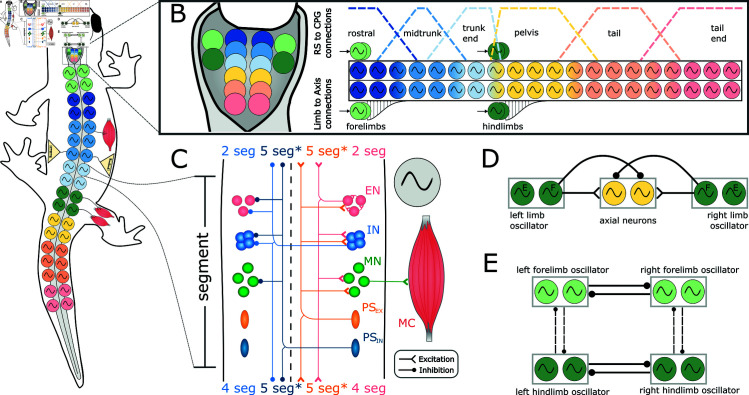
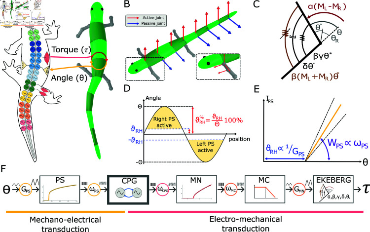
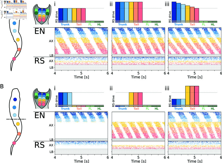
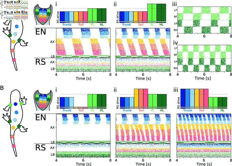
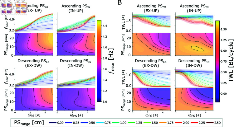
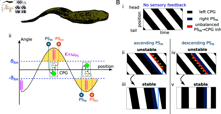
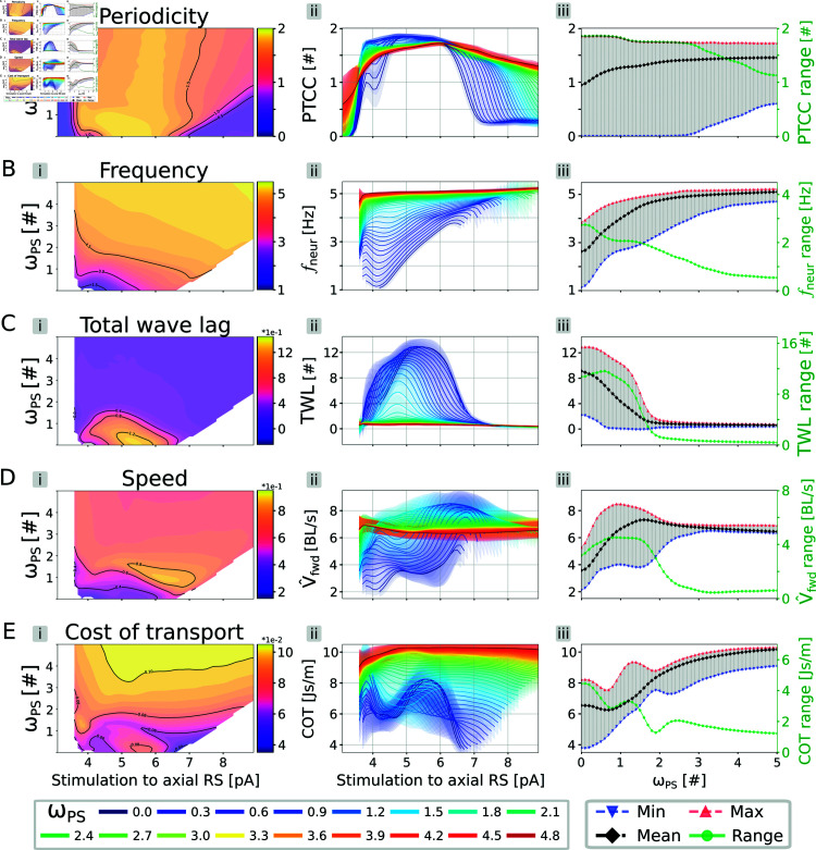
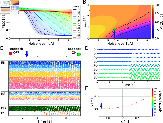
This study introduces a novel neuromechanical model employing a detailed spiking neural network to explore the role of axial proprioceptive sensory feedback, namely stretch feedback, in salamander locomotion. Unlike previous studies that often oversimplified the dynamics of the locomotor networks, our model includes detailed simulations of the classes of neurons that are considered responsible for generating movement patterns. The locomotor circuits, modeled as a spiking neural network of adaptive leaky integrate-and-fire neurons, are coupled to a three-dimensional mechanical model of a salamander with realistic physical parameters and simulated muscles. In open-loop simulations (i.e., without sensory feedback), the model replicates locomotor patterns observed in-vitro and in-vivo for swimming and trotting gaits. Additionally, a modular descending reticulospinal drive to the central pattern generation network allows to accurately control the activation, frequency and phase relationship of the different sections of the limb and axial circuits. In closed-loop swimming simulations (i.e. including axial stretch feedback), systematic evaluations reveal that intermediate values of feedback strength increase the tail beat frequency and reduce the intersegmental phase lag, contributing to a more coordinated, faster and energy-efficient locomotion. Interestingly, the result is conserved across different feedback topologies (ascending or descending, excitatory or inhibitory), suggesting that it may be an inherent property of axial proprioception. Moreover, intermediate feedback strengths expand the stability region of the network, enhancing its tolerance to a wider range of descending drives, internal parameters' modifications and noise levels. Conversely, high values of feedback strength lead to a loss of controllability of the network and a degradation of its locomotor performance. Overall, this study highlights the beneficial role of proprioception in generating, modulating and stabilizing locomotion patterns, provided that it does not excessively override centrally-generated locomotor rhythms. This work also underscores the critical role of detailed, biologically-realistic neural networks to improve our understanding of vertebrate locomotion.

Fig 1. Neural model.

A) shows the schematics of the locomotor network organization. The axial network is comprised of two chains of oscillators (i.e., the hemisegments), divided into 40 equivalent segments (only a fraction is shown). The axial segments are spatially organized in trunk and tail sub-networks. In correspondence of the two girdles (green oscillator symbols) there are the equivalent segments for the limb networks. Each segment projects to a pair of antagonist muscle cells. The axial network receives proprioceptive sensory feedback (PS) based on the local curvature of the model. The limb network does not receive sensory feedback. B) shows the organization of the reticulosponal population (RS). The axial RS neurons are divided into 6 sub modules (3 for the trunk, 3 for the tail) projecting to the axial central pattern generator (CPG) neurons according to overlapping trapezoidal distributions, shown as dotted lines. The limb RS neurons are divided into 4 modules, each projecting to a separate limb segment. The limb segments project to the axial CPG network with local (i.e.; spanning few segments) descending distributions. C) shows the organization of each equivalent segment of the CPG network. The structure comprises excitatory (EN) and inhibitory (IN) CPG neurons, motoneurons (MN), excitatory (PS_EX) and inhibitory (PS_IN) proprioceptive sensory neurons and muscle cells (MC). Only a fraction of the neurons and their connections originating from the right hemisegment are shown. The connections from the left hemisegment follow the same organization principle. The range of the ascending and descending projections is displayed in terms of equivalent segments (seg). The PS connection ranges (indicated with an asterisk *) were modified in the following analyses to investigate the effect of feedback topology (excitation/inhibition, ascending/descending) on the closed-loop network. D) shows the limb-to-body connectivity pattern. Each flexor (i.e. protractor) hemisegment of a limb oscillator excites the ipsilateral axial hemisegments and inhibits the contralateral axial hemisegments. E) shows the inter-limb connectivity scheme. Each limb oscillator sends inhibitory projections from the flexor side to the flexor side of the commissural and ipsilateral limbs. The commissural connections (thick lines) are stronger than the ipsilateral projections (dotted lines) to ensure the left-rialternation between opposed forelimbs and hindlimbs.

Fig 2. Mechanical model.

A) shows the exchange of information between the neural and mechanical model. The neural model sends torque commands to the joints and reads back the corresponding joint angles. B) shows the active (in red) and passive (in blue) joints of the axial body. Active joints exert their action in the horizontal plane. Passive joints excert their action in the sagittal plane. The insert shows the active degrees of freedom of each limb. The shoulder and hip joints are spherical joints allowing rotations about the three axes. The elbow and knee joints are hinge joints that allow flexion/extension. C) displays the equivalent scheme of an Ekeberg muscle model. It is a rotational spring-damper system with the addition of a variable stiffness term β ( M_L + M_R ) θ^*. The active term of the model acts an external torque α ( M_L - M_R ) . D) shows the relationship between the joint angles (θ) and the corresponding proprioceptive sensory neurons activity (PS). When θ crosses a threshold value θ_RH (i.e.; the rheobase angle) the PS neurons on the stretched side become active (yellow area). Notably, the ratio (in percentage) between each joint’s oscillation amplitude (Θ) and the corresponding threshold θ_RH is constant along the entire axial network and it is equal to ${\theta }_{RH}^{\%}$. E) shows the equivalent scheme for the mechano-electrical transduction principle, in analogy with proportional control. The rheobase angle θ_RH indicates the critical angle for which the PS neurons become active. The feedback synaptic weight ω_PS modulates the strength W (i.e., the slope) of the PS action once θ_RH is crossed. F) displays the control diagram for the mechano-electrical and electro-mechanical transduction. The axial central pattern generators (CPGs) receive curvature information through the PS population. The activity of the CPGs is translated into torque information through the Ekeberg muscle model via motoneurons (MN) and muscle cells (MC).

Fig 3. Open loop swimming network.

A) shows the swimming pattern emerging from three different levels of stimulation to the axial RS. The level of stimulation provided to the 10 RS modules (6 axial, 4 limbs) is shown on top of each plot. The raster plots represent the spike times of excitatory neurons (EN) and reticulospinal neurons (RS). For the axial network (AX), only the activity of the left side is displayed. For the limb network (LB), only the activity of the flexor side is displayed. Limbs are ordered as left forelimb (LF), right forelimb (RF), left hindlimb (LH), right hindlimb (RH), from top to bottom. Ai shows the pattern obtained with a constant drive of 5.0pA. The neural activity corresponds to a frequency f_neur = 2 . 1Hz and a total wave lag TWL = 1 . 04. Aii shows the response to a higher constant drive of 5.7pA. The neural activity corresponds to f_neur = 3 . 1Hz and TWL = 1 . 27. Aiii shows the effect of driving the network with a gradient of excitation ranging from 5.7pA (to the rostral RS neurons) to 5.0pA (to the tail RS neurons). The neural activity corresponds to f_neur = 3 . 1Hz and TWL = 1 . 83. B) shows the coordination patterns achieved for different levels of stimulation to the trunk and tail regions. Bi shows the activity corresponding to a stimulation of 5.7pA of the trunk RS. The trunk network is rhythmically active, but the activity does not spread to the tail network. Bii shows the activity corresponding to a stimulation of 5.7pA of the tail RS. The tail network is rhythmically active, but the activity does not spread to the trunk network. Biii shows the activity corresponding to a different level stimulation of the trunk (5.0pA) and tail (6.2pA) RS neurons. Both regions are rhythmically active and the tail network oscillates at a higher frequency with a 2:1 ratio with respect to the trunk network.

Fig 4. Open loop walking network.

A) shows the walking pattern emerging from different levels of stimulation to the axial and limb RS. The level of stimulation provided to the 10 RS modules (6 axial, 4 limbs) is shown on top of each plot. The raster plots represent the spike times of every neuron of the spinal cord model. For the axial network (AX), only the activity of the left side is displayed. For the limb network (LB), only the activity of the flexor side is displayed. Limbs are ordered as left forelimb (LF), right forelimb (RF), left hindlimb (LH), right hindlimb (RH), from top to bottom. Ai shows the pattern obtained with a constant drive to the limbs and axial RS with an amplitude of 5.0pA and 4.0pA, respectively. The neural activity corresponds to f_neur = 0 . 8Hz. Aii shows the response to a higher constant drive of 5.5pA to the limb RS. The neural activity corresponds to f_neur = 1 . 3Hz. Aiii and Aiv show the limb activity recorded during the experiments in Ai and Aii, respectively. B) shows the coordination patterns achieved when modulating the drive to the axial RS modules. Bi shows the response of the network from Aii when the tail RS modules do not receive any drive. The tail network remains silent. Bii shows the response of the network from Aii when the tail RS modules receive an increased drive of 6.5pA. The tail network oscillates at a higher frequency with a 2:1 ratio with respect to the trunk network. Biii shows the response of the network with an axial RS drive of 6.0pA and a limbs RS drive of 4.5pA. The axial network displays a travelling wave of activity despite the rhythmic limb activation.

Fig 5. Frequency and phase lag modulation during swimming with different sensory feedback topologies and strengths.

Panels A and B show the effect of different PS topology patterns and weights on the frequency (f_neur) and total wave lag (TWL) of the network’s activity, respectively. The studied topologies include ascending excitation (EX-UP), descending excitation (EX-DW), ascending inhibition (IN-UP) and descending inhibition (IN-DW). The range of the connections (PS range) was varied in the range  [ 0 , 2 . 5 ] mm (i.e., between 0 and 10 equivalent segments). Similarly, the PS synaptic weight (ω_PS) was varied in the range  [ 0 , 5 ] . The rheobase angle ratio was set to ${\theta }_{RH}^{\%}=10\%$. A) shows the modulation of the oscillations’ frequency (f_neur). In each quadrant, the contour plot shows the dependency of the f_neur on PS range and ω_PS. On top, the projection of the relationship in the f_neur - ω_PS plane is displayed to better highlight the asymptotical values reached by f_neur. The different curves represent the frequency expressed by the network with different PS connection ranges (i.e.; horizontal cuts of the contour plot), whose value is reported in the legend. The thick lines represent the mean metric values across 20 instances of the network, built with different seeds for the random number generator. The shaded areas represent one standard deviation of difference from the mean. B) follows the same organization as the previous panel to represent the effect of feedback topology on the neural total wave lag (TWL).

Fig 6. Illustrative diagrams showing the mechanism of frequency and phase lag control by stretch feedback.

A)i shows a sketch of a sinusoidal-like body curvature during swimming. Aii shows populations of CPG and PS neurons at the location of maximal curvatures and their connections (active population have filled colors, inactive populations have white inner colors). The activity of PS neurons in correspondence of large curvatures (above θ_RH) acts as an equivalent spring that induces an increase of the swimming frequency. The figure is drawn for ${\theta }_{RH}^{\%}=40\%$ to better highlight the components of the network. B) shows the stereotypical CPG activities during swimming in a brief time window (black=active/firing, white=inactive) sorted according to the CPG positions (top=head positions, bottom=tail positions). Bi shows the activities of CPGs with no feedback (in open loop). Bii-Bv also show the activities of CPGs and left proprioceptive PS_IN neurons (dark blue) in closed loop. The sub-panels Bii-Biii and Biv-Bv show subsequent time-windows at starting and final stages of activities from the time when inhibitory proprioceptive sensory feedback (PS_IN) is turned on. The light blue arrows represent the PS_IN projections in the ascending (Bii-Biii) and descending (Biv-v) directions to the closest CPG neurons on the opposite sides, respectively. These indicate the end/start of a region of unbalanced (i.e.; not uniformly distributed across the network) inhibition from PS_IN to the CPGs (red areas). This imbalance in PS_IN inhibition causes a delay shift in the activations of the corresponding CPGs according to the direction indicated by the yellow arrows. See the text for more details.

Fig 7. Intermediate feedback strengths improve the performance of the closed loop swimming network.

In each panel, the stimulation amplitude to the axial RS neurons was varied in the range  [ 3 . 0 , 9 . 0 ] pA, while the feedback weight (ω_PS) was varied in the range  [ 0 . 0 , 5 . 0 ] . The rheobase angle ratio was set to ${\theta }_{RH}^{\%}=10\%$. The displayed data is averaged across 20 instances of the network, built with different seeds for the random number generator. In Aii-Eii, the curves differ by their corresponding value of ω_PS, reported in the bottom legend. The shaded areas represent one standard deviation of difference from the mean. In Aiii-Eiii, the minimum (in blue), maximum (in red) average (in black) and range (in green) for the corresponding metrics across all the considered stimulation values are shown. The range values are reported on the y-axis on the right. Panels (A-E) display the effect on the network’s periodicity (PTCC), frequency (f_neur), total wave lag (TWL), speed (V_fwd) and cost of transport (COT), respectively. In panels B-E, combinations with PTCC < 1 were not displayed.

Fig 8. Effect of noise on the closed loop swimming network.

A) shows the effect of noise amplitude on the rhythmicity of the network (PTCC) with different levels of sensory feedback weight (ω_PS). The noise level was varied in the range  [ 3 . 0 , 9 . 5 ]  pA. The feedback weight was varied in the range  [ 0 . 0 , 3 . 0 ] . The rheobase angle ratio was set to ${\theta }_{RH}^{\%}=10\%$. The different curves represent the average PTCC values across 20 instances of the network (built with different seeds for the random number generator) for different levels of ω_PS (shown in the legend). The shaded areas represent one standard deviation of difference from the mean. B) displays the noise-feedback relationship in 2D. For a noise level of 5.6 pA, increasing ω_PS from 0 (red dot) to 0.7 (green point) leads to a switch from irregular to organized rhythmic activity. C) shows the switch effect with a noise level of 5.6 pA. The raster plot represents the spike times of excitatory neurons (EN), reticulospinal neurons (RS), motoneurons (MN) and proprioceptive sensory neurons (PS). Only the activity of the left side of the network is displayed. At time = 2.5 s (blue arrow), the sensory feedback weight is changed from ω_PS = 0 (Feedback OFF) to ω_PS = 0 . 7 (Feedback ON), restoring a left-right alternating rhythmic network activity. D) shows the axial joint angles during the simulation in C. Each angle is shown in the range  [ - 25^∘ , + 25^∘ ] . E) shows the center of mass trajectory during the simulation in C. Activating feedback restored forward swimming.

Fig 9. Sensory feedback extends the rhythmogenic capabilities of the network.

A) shows the dependency of the periodicity (PTCC) on the inhibition strength and on the feedback weight (ω_PS) for the swimming network. The commissural inhibition strength was varied in the range  [ 0 . 0 , 6 . 0 ] . The feedback weight was varied in the range  [ 0 . 0 , 5 . 0 ] . The rheobase angle ratio was set to ${\theta }_{RH}^{\%}=10\%$. The displayed values are averaged across 20 instances of the network, built with different seeds for the random number generator. B) shows the inhibition-feedback relationship in 1D. The different curves represent the average PTCC values for different levels of ω_PS (shown in the legend). The shaded areas represent one standard deviation of difference from the mean. Panels C and D follow the same organization as the previous panels to highlight the inhibition-feedback relationship for ω_PS values in the range  [ 0 . 0 , 1 . 0 ] .

References

1. Grillner S, El Manira A. current principles of motor control, with special reference to vertebrate locomotion. Physiol Rev 2020;100(1):271–320. doi: 10.1152/physrev.00015.2019 - DOI - PubMed
1. Wallén P, Ekeberg O, Lansner A, Brodin L, Tråvén H, Grillner S. A computer-based model for realistic simulations of neural networks. II. The segmental network generating locomotor rhythmicity in the lamprey. J Neurophysiol 1992;68(6):1939–50. doi: 10.1152/jn.1992.68.6.1939 - DOI - PubMed
1. Hellgren J, Grillner S, Lansner A. Computer simulation of the segmental neural network generating locomotion in lamprey by using populations of network interneurons. Biol Cybern 1992;68(1):1–13. doi: 10.1007/BF00203132 - DOI - PubMed
1. Kozlov A, Huss M, Lansner A, Kotaleski JH, Grillner S. Simple cellular and network control principles govern complex patterns of motor behavior. Proc Natl Acad Sci 2009;106(47):20027–32. doi: 10.1073/pnas.0906722106 - DOI - PMC - PubMed
1. Dubuc R, Cabelguen J-M, Ryczko D. Locomotor pattern generation and descending control: a historical perspective. J Neurophysiol 2023;130(2):401–16. doi: 10.1152/jn.00204.2023 - DOI - PubMed
LinkOut - more resources