Dendrites endow artificial neural networks with accurate, robust and parameter-efficient learning

Abstract

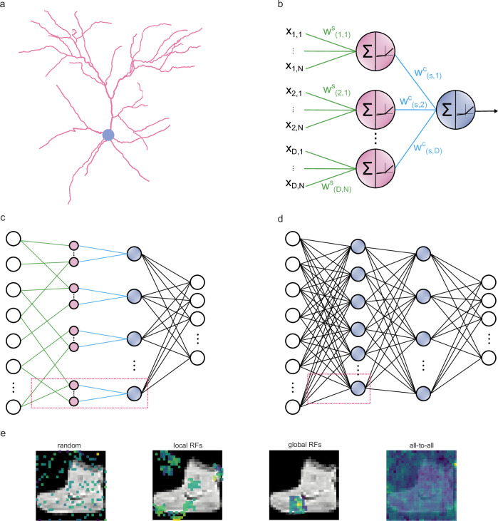
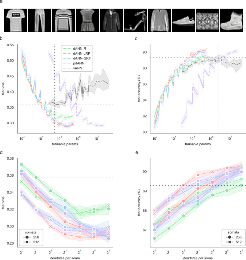
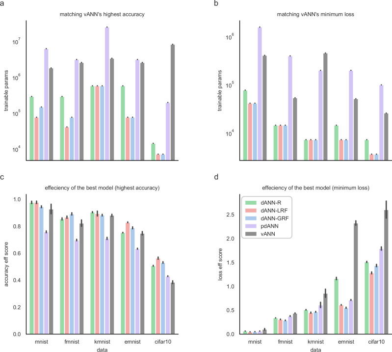
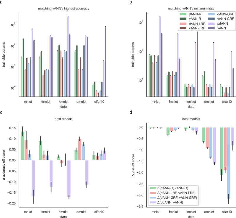
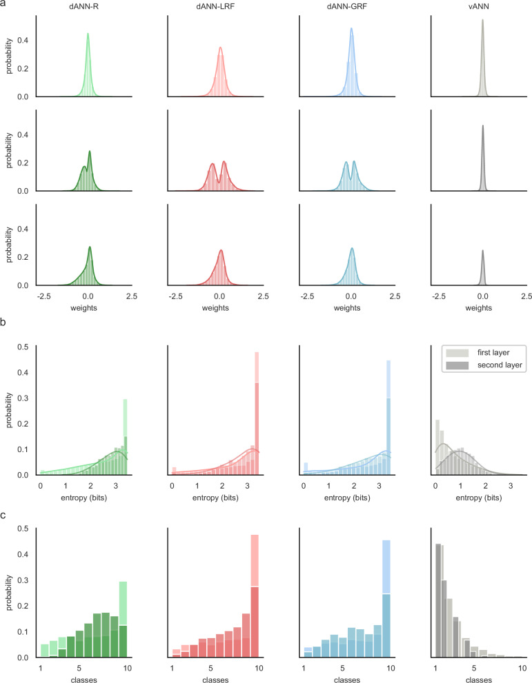
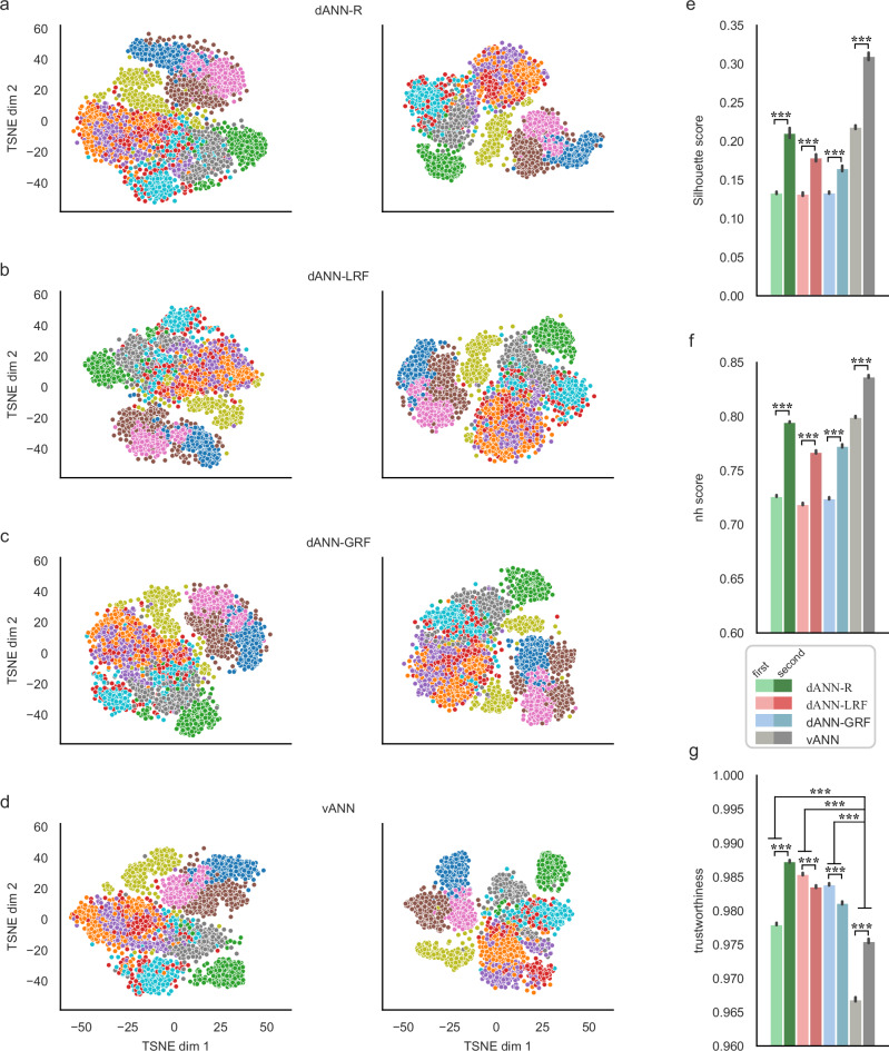
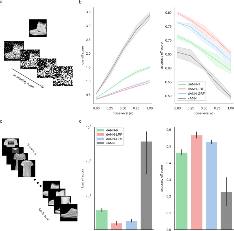
Artificial neural networks (ANNs) are at the core of most Deep Learning (DL) algorithms that successfully tackle complex problems like image recognition, autonomous driving, and natural language processing. However, unlike biological brains who tackle similar problems in a very efficient manner, DL algorithms require a large number of trainable parameters, making them energy-intensive and prone to overfitting. Here, we show that a new ANN architecture that incorporates the structured connectivity and restricted sampling properties of biological dendrites counteracts these limitations. We find that dendritic ANNs are more robust to overfitting and match or outperform traditional ANNs on several image classification tasks while using significantly fewer trainable parameters. These advantages are likely the result of a different learning strategy, whereby most of the nodes in dendritic ANNs respond to multiple classes, unlike classical ANNs that strive for class-specificity. Our findings suggest that the incorporation of dendritic properties can make learning in ANNs more precise, resilient, and parameter-efficient and shed new light on how biological features can impact the learning strategies of ANNs.

Fig. 1. Schematic representation of the dendritic ANN (dANN) compared to a classical vanilla ANN (vANN).

a Example of a layer 2/3 pyramidal cell of the mouse primary visual cortex (dendrites: pink; soma: grey) that served as inspiration for the artificial dendritic neuron in b. The morphology was adopted from Park et al.. b The dendritic neuron model consists of a somatic node (blue) connected to several dendritic nodes (pink). All nodes have a nonlinear activation function. Each dendrite is connected to the soma with a (cable) weight, w_(d,s)^c, where d and s denote the dendrite and soma indices, respectively. Inputs are connected to dendrites with (synaptic) weights, w_(d,n)^s, where d and n are indices of the dendrites and input nodes, respectively. dϵ{1, D}, nϵ{1, N}, N denotes the number of synapses each dendrite receives, and D the number of dendrites per soma s. c The dendritic ANN architecture. The input is fed to the dendritic layer (pink nodes), passes a nonlinearity, and then reaches the soma (blue nodes), passing through another nonlinearity. Dendrites are connected solely to a single soma, creating a sparsely connected network. d Typical fully connected ANN with two hidden layers. Nodes are point neurons (blue) consisting only of a soma. e Illustration of the different strategies used to sample the input space: random sampling (R), local receptive fields (LRF), global receptive fields (GRF), and fully connected (F) sampling of input features. Examples correspond to the synaptic weights of all nodes that are connected to the first unit in the second layer. The colormap denotes the magnitude of each weight. The image used in the background is from the Fashion MNIST (FMNIST) dataset (see Methods).

Fig. 2. Dendritic features improve learning on Fashion MNIST classification.

a The Fashion MNIST dataset consists of 28×28 grayscale images of 10 categories. b Average test loss as a function of the trainable parameters of the five models used: A dendritic ANN with random inputs (dANN-R, green), a dANN with LRFs (red), a dANN with GRFs (blue), a partly-dendritic ANN with all-to-all inputs (pdANN, purple), and the vANN with all-to-all inputs (grey). Horizontal and vertical dashed lines denote the minimum test loss of the vANN and its trainable parameters, respectively. The x-axis is shown in a logarithmic scale (log10). c Similar to B, but depicting the test accuracy instead of the loss. d Test loss as a function of the number of dendrites per somatic node for the three dANNs and the pdANN model. The linestyle (solid and dashed) represents different somatic numbers. The dashed horizontal line represents the minimum test loss of the vANN (512-256 size of its hidden layers, respectively). The x-axis is shown in a logarithmic scale (log2). e Similar to (d), but showing the test accuracy instead of the loss. The dashed horizontal line represents the maximum test accuracy of the vANN (2048-512 size of its hidden layers, respectively). Note that while all models have the same internal connectivity structure, the pdANN model (purple) has a much larger number of trainable parameters due to its all-to-all input sampling. For all panels, shades represent the 95% confidence interval across N = 5 initializations for each model.

Fig. 3. Dendrites improve efficiency across various benchmark datasets.

The comparison is made between the three dendritic models, dANN-R (green), dANN-LRF (red), dANN-GRF (blue), the partly-dendritic model pdANN (purple) and the vANN (grey). a Number of trainable parameters that each model needs to match the highest test accuracy of the vANN. b The same as in a, but showing the number of trainable parameters required to match the minimum test loss of the vANN. c Accuracy efficiency scores of all models across the five datasets tested. This score reports the best test accuracy achieved by a model, normalized with the logarithm of the product of trainable parameters with the number of epochs needed to achieve minimum validation loss. The score is bounded in [0, 1]. d Same as in c, but showing the loss efficiency score. Here the minimum loss achieved by a model is normalized with the logarithm of the trainable parameters times the number of epochs needed to achieve minimum validation loss. The score is bounded in [0, ∞). In all barplots the error bars represent one standard deviation across N = 5 initializations for each model.

Fig. 4. Comparison of dendritic, partly-dendritic, and vanilla ANNs with different types of input sampling.

The following models were compared: dANN-R and vANN-R with random input sampling (light and dark green), dANN-LRF and vANN-LRF with local receptive field sampling (light and dark red), dANN-GRF and vANN-GRF with global receptive field sampling (light and dark blue), and pdANN and vANN with all-to-all sampling (light and dark purple). a Number of trainable parameters that each model needs to match the highest test accuracy of the respective vANN. b The same as in a, but showing the number of trainable parameters required to match the minimum test loss of the vANN. c Difference (Δ) in accuracy efficiency score between the structured (dANN/pdANN) and vANN models. Test accuracy is normalized with the logarithm of trainable parameters times the number of epochs needed to achieve minimum validation loss. The score is bounded in [0, 1]. d Same as in c, but showing the difference (Δ) of the loss efficiency score. Again, we normalized the test score with the logarithm of the trainable parameters times the number of epochs needed to achieve minimum validation loss. The score is bounded in [0, ∞). In all barplots the error bars represent one standard deviation across N = 5 initializations for each model.

Fig. 5. Dendritic ANN models fully exploit their available resources and solve the task using a different learning strategy.

a Weight probability density functions after training for dANN-R, dANN-GRF, dANN-LRF, and vANN. The density functions are built by concatenating all weights across N = 5 initializations for each model. First hidden layer (top row), second hidden layer (middle row), and output layer (bottom row) weights are shown. Both x and y axes are shared across all subplots for visual comparison among the density plots. Supplementary Table 2 contains the kurtosis, skewness, and range of all KDE plots. b Probability density function of the entropy (bits) for the first (normal color) and second (shaded color) hidden layer, respectively. Entropies are calculated using the activations of each layer for all test images of FMNIST (see Methods). Silent nodes have been excluded from the visualization. Higher values signify mixed selectivity, whereas low values indicate class specificity. c Probability density functions of selectivity for both layers (different color shades) and all models (columns). For all histograms, the bins are equal to the number of classes, i.e., for the FMNIST dataset.

Fig. 6. Learned representations.

a–d TSNE projections of the activations for the first (left column) and the second (right column) hidden layers corresponding to the three dANN and the vANN models. Different colors denote the image categories of the FMNIST dataset. While the figure shows the results of one run, the representations are consistent across 10 runs of the TSNE algorithm (data not shown). e Silhouette scores of the representations (2-way ANOVA: model F(3,32) = 1598.31, p < 10⁻³, layer F(1,32) = 2130.39, p < 10⁻³, model x layer F(3,32) = 105.20, p < 10⁻³). f Neighborhood scores of the representations, calculated using 11 neighbors (2-way ANOVA: model F(3,32) = 8624.78, p < 10⁻³, layer F(1, 32) = 18512.42, p < 10⁻³, model x layer F(3, 32) = 299.51, p < 10⁻³). g Trustworthiness of the representations, calculated using 11 neighbors (2-way ANOVA: model F(3,32) = 6187.66, p < 10⁻³, layer F(1,32) = 1856.84, p < 10⁻³, model x layer F(3,32) = 1777.98, p < 10⁻³). In all barplots the error bars represent the 95% confidence interval across N = 5 initializations for each model and 10 runs of the TSNE algorithm per initialization. Stars denote significance with unpaired t-test (two-tailed) with Bonferroni’s correction.

Fig. 7. Dendritic ANNs are more accurate and efficient than vANNs when inputs are noisy or presented in a sequential manner.

a An example of one FMNIST image with variable Gaussian noise. Sigma (σ) is the standard deviation of the Gaussian noise. b Testing loss (left) and accuracy (right) efficiency scores for all models and noise levels. Shades represent one standard deviation across N = 5 network initializations for each model. c The sequential learning task. d As in (b), but showing the loss (left) and accuracy (right) efficiency scores for the sequential task. Errorbars denote one standard deviation across N = 5 initializations for each model. See Table 2 and Supplementary Table 3 for the accuracy and loss values.

References

1. Attwell, D. & Laughlin, S. B. An energy budget for signaling in the grey matter of the brain. J. Cereb. Blood Flow Metab.21, 1133–1145 (2001). - PubMed
1. Luccioni, A. S., Jernite, Y. & Strubell, E. Power hungry processing: watts driving the cost of AI deployment? In Proc.2024 ACM Conference on Fairness, Accountability, and Transparency 85–99 (FACCT, 2024).
1. Strubell, E., Ganesh, A. & McCallum, A. Energy and policy considerations for deep learning in NLP. In Proc. 57th Annual Meeting of the Association for Computational Linguistics, 3645–3650 (Association for Computational Linguistics, Florence, Italy, 2019).
1. Mehonic, A. & Kenyon, A. J. Brain-inspired computing needs a master plan. Nature604, 255–260 (2022). - PubMed
1. McCloskey, M. & Cohen, N. J. Catastrophic interference in connectionist networks: the sequential learning problem. in Psychology of Learning and Motivation vol. 24 109–165 (Elsevier, 1989).
LinkOut - more resources