Impact of Varying Sleep Pressure on Daytime Sleep Propensity in Healthy Young and Older Adults

Abstract

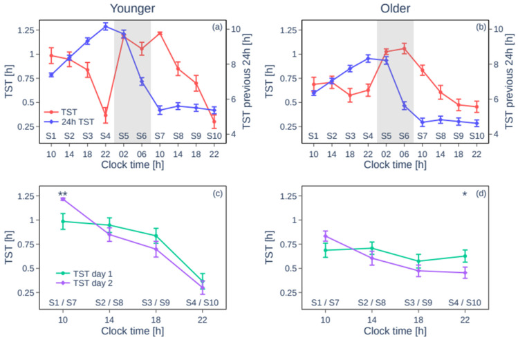
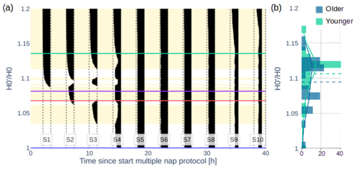
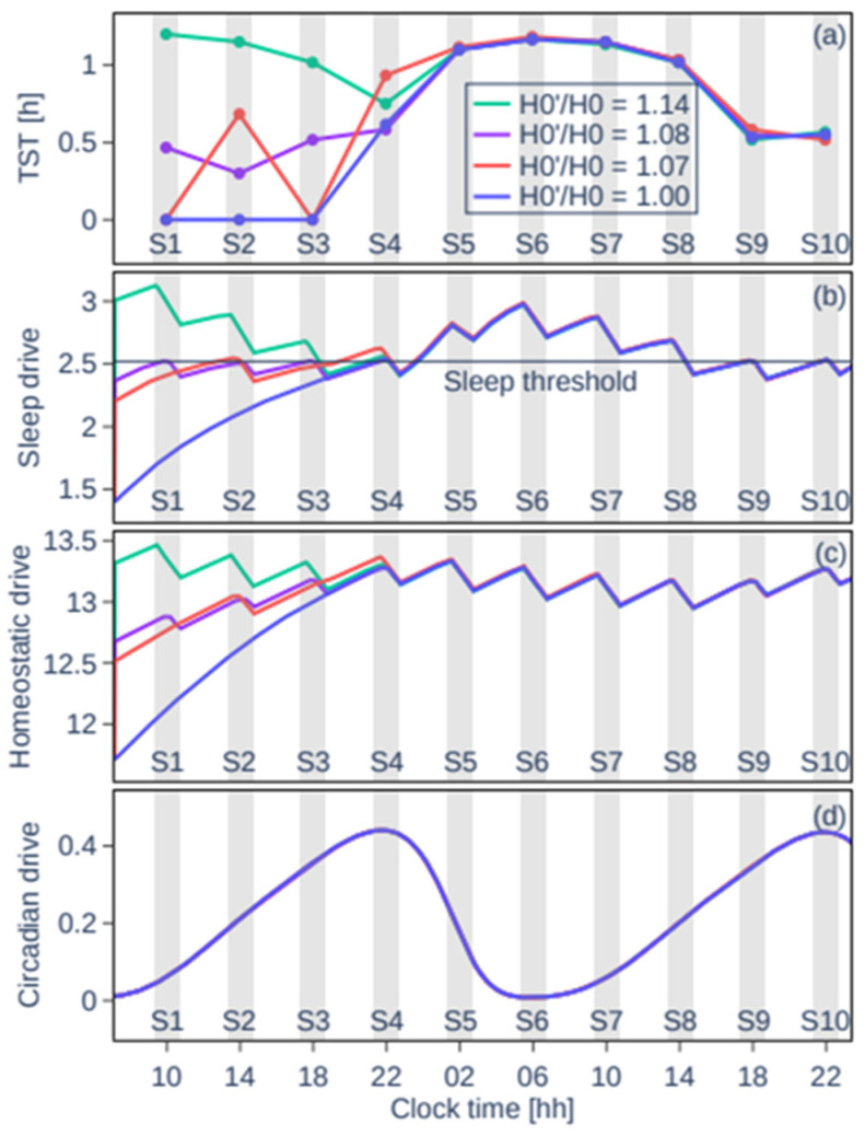
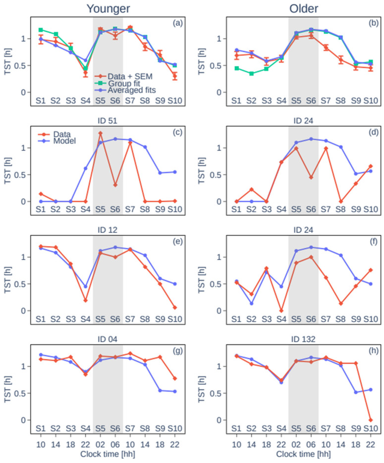
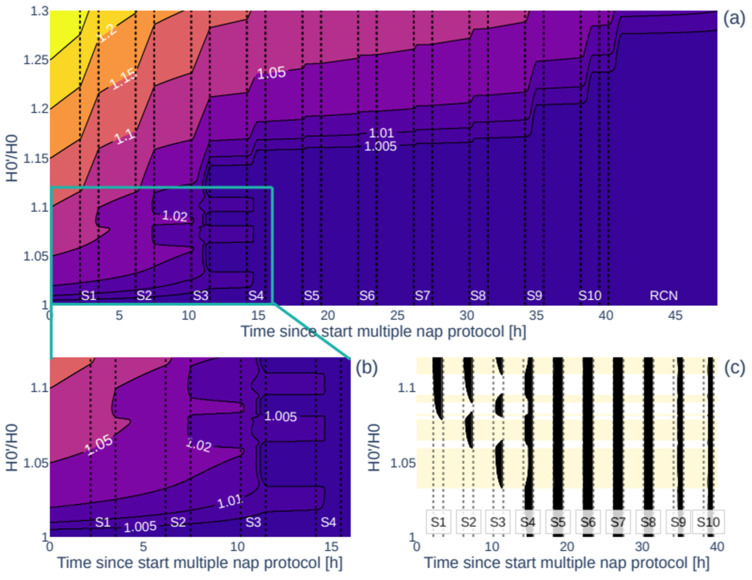
Fixed sleep schedules with an 8 h time in bed (TIB) are used to ensure participants are well-rested before laboratory studies. However, such schedules may lead to cumulative excess wakefulness in young individuals. Effects on older individuals are unknown. We combine modelling and experimental data to quantify the effects of sleep debt on sleep propensity in healthy younger and older participants. A model of arousal dynamics was fitted to sleep data from 22 young (20-31 y.o.) and 26 older (61-82 y.o.) individuals (25 male) undertaking 10 short sleep-wake cycles during a 40 h napping protocol, following >1 week of fixed 8 h TIB schedules. Homeostatic sleep drive at the study start was varied systematically to identify best fits between observed and predicted sleep profiles for individuals and group averages. Daytime sleep duration was the same on the two days of the protocol within the groups but different between the groups (young: 3.14 ± 0.98 h vs. 3.06 ± 0.75 h, older: 2.60 ± 0.98 h vs. 2.37 ± 0.64 h). The model predicted an initial homeostatic drive of 11.2 ± 3.5% (young) and 10.1 ± 3.5% (older) above well-rested. Individual variability in first-day, but not second-day, sleep patterns was explained by the differences in the initial homeostatic drive for both age groups. Our study suggests that both younger and older participants arrive at the laboratory with cumulative sleep debt, despite 8 h TiB schedules, which dissipates after the first four sleep opportunities on the protocol. This has implications for protocol design and the interpretation of laboratory studies.

Keywords: ageing; homeostatic pressure; modelling; napping; sleep; sleep debt; sleep propensity.

Figure 1

Sleep duration and sleep history over the multiple nap protocol. The top panels show the group mean total sleep time (TST) per sleep opportunity (red) and mean cumulative sleep time over the prior 24 h (blue) (±SEM) throughout the protocol. The bottom panels compare the TSTs during the sleep opportunities appearing at the same clock time on the first (S1–S4) and the second (S7–S10) day (with significant differences indicated with * for p < 0.05 and ** for p < 0.01). Panels (a,c) are for the younger group, and (b,d) are for the older group. Clock times are averaged protocol times.

Figure 2

Effect of the initial homeostatic drive on sleep patterns on the multiple nap protocol. (a) Modelled sleep–wake pattern (with sleep in black and wake in white/yellow) over the 40 h multiple nap protocol as a function of the initial homeostatic drive H₀′/H₀. For H₀′/H₀ = 1, no sleep debt is introduced, and no sleep occurs in S1–S3 (blue line). Increasing H₀′/H₀ changes the sleep–wake pattern in S1–S4 and increases the TST over the protocol. The alternating yellow and white background colours indicate the areas with distinct sleep–wake patterns. The coloured lines correspond to the time courses of Figure 3. (b) Histogram of the best fit H₀′/H₀ values for the younger and older participants.

Figure 3

Time courses from the arousal dynamics model during the 40 h multiple nap protocol. For four different initial homeostatic drives: no sleep debt (blue), a low sleep debt (red), slightly higher sleep debt (purple), and a high sleep debt (green). (a) The TST shows four distinct modelled sleep behaviour patterns. (b) The sleep drive determines that sleep will occur when the sleep threshold is reached during a sleep opportunity. A slight variation in sleep drive can result in very different sleep profiles. The sleep drive consists of the homeostatic drive (c), the circadian drive (d), and a constant. (c) The homeostatic drive is modified to model the sleep debt at the start of the protocol. (d) The circadian drive is not affected by the sleep debt.

Figure 4

Total sleep times and model fits for group average data and representative individuals. Panels (a,b) show the group mean TST per sleep opportunity over the protocol with the SEM (red), the group mean fit (green), and the mean of the individual fits (blue). Left panels show data for younger participants and right panels show data for older participants. Panels (c,d) show participants with little sleep debt, panels (e,f) show participants with average sleep debt, and panels (g,h) show participants with large sleep debt.

Figure 5

Wash-out effect of sleep debt during the multiple nap protocol. (a) A contour map demonstrating the effects of the initial homeostatic drive H₀′/H₀ and time into protocol on the dynamics of H’/H—the homeostatic variable H’ relative to its default value, H. Darker colour indicates a smaller H’/H value with H’/H = 1 indicating that H’ converged to H and the effect of the initial sleep debt is no longer present. (b) Zoomed in section of the contour map in (a). (c) Corresponding sleep–wake pattern. The alternating white and yellow background colours indicate the different modes as separated by the sleep thresholds.

References

1. Borbely A.A. A Two Process Model of Sleep Regulation. Hum. Neurobiol. 1982;1:195–204. - PubMed
1. Daan S., Beersma D.G., Borbély A.A. Timing of Human Sleep: Recovery Process Gated by a Circadian Pacemaker. Am. J. Physiol. 1984;246:R161–R183. doi: 10.1152/ajpregu.1984.246.2.R161. - DOI - PubMed
1. Edgar D., Dement W., Fuller C. Effect of SCN Lesions on Sleep in Squirrel Monkeys: Evidence for Opponent Processes in Sleep-Wake Regulation. J. Neurosci. 1993;13:1065–1079. doi: 10.1523/JNEUROSCI.13-03-01065.1993. - DOI - PMC - PubMed
1. Borbély A.A., Achermann P. Chapter 33—Sleep Homeostasis and Models of Sleep Regulation. In: Kryger M.H., Roth T., Dement W.C., editors. Principles and Practice of Sleep Medicine (Fourth Edition) W.B. Saunders; Philadelphia, PA, USA: 2005. pp. 405–417.
1. Dijk D.J., Czeisler C.A. Paradoxical Timing of the Circadian Rhythm of Sleep Propensity Serves to Consolidate Sleep and Wakefulness in Humans. Neurosci. Lett. 1994;166:63–68. doi: 10.1016/0304-3940(94)90841-9. - DOI - PubMed
LinkOut - more resources