Longitudinal phage-bacteria dynamics in the early life gut microbiome

Abstract

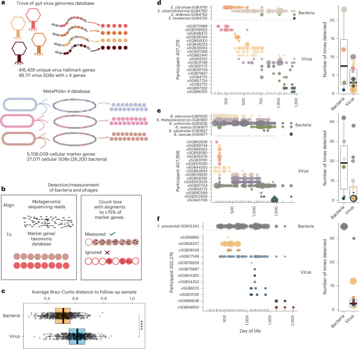
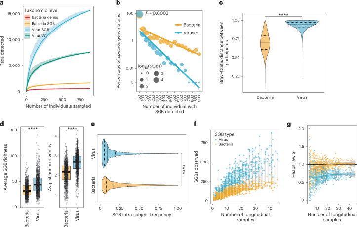
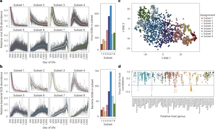
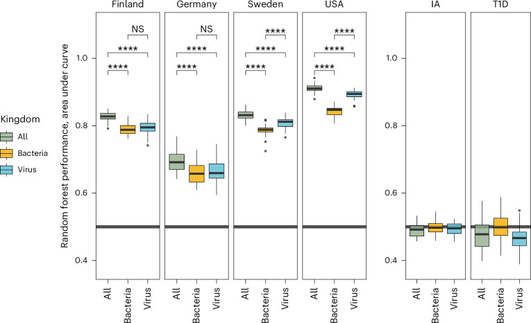
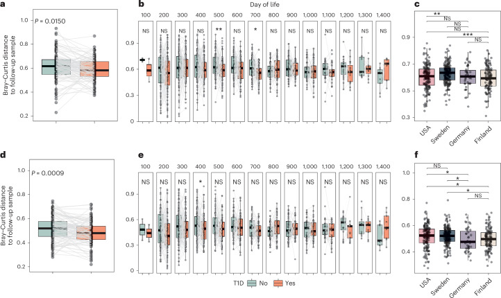
Microbial colonization of the human gut occurs soon after birth, proceeds through well-studied phases and is affected by lifestyle and other factors. Less is known about phage community dynamics during infant gut colonization due to small study sizes, an inability to leverage large databases and a lack of appropriate bioinformatics tools. Here we reanalysed whole microbial community shotgun sequencing data of 12,262 longitudinal samples from 887 children from four countries across four years of life as part of the The Environmental Determinants of Diabetes in the Young (TEDDY) study. We developed an extensive metagenome-assembled genome catalogue using the Marker-MAGu pipeline, which comprised 49,111 phage taxa from existing human microbiome datasets. This was used to identify phage marker genes and their integration into the MetaPhlAn 4 bacterial marker gene database enabled simultaneous assessment of phage and bacterial dynamics. We found that individual children are colonized by hundreds of different phages, which are more transitory than bacteria, accumulating a more diverse phage community over time. Type 1 diabetes correlated with a decreased rate of change in bacterial and viral communities in children aged one and two. The addition of phage data improved the ability of machine learning models to discriminate samples by country. Finally, although phage populations were specific to individuals, we observed trends of phage ecological succession that correlated well with putative host bacteria. This resource improves our understanding of phage-bacteria interactions in the developing early life microbiome.

Fig. 1. Marker-MAGu enables trans-kingdom taxonomic profiling of gut metagenomes.

a, Schematic of the Marker-MAGu database structure. b, Marker-MAGu profiling ruleset. c, Average Bray–Curtis dissimilarity between adjacent samples for all participants with at least ten samples for virome and bacteriome (n = 566). ****P < 1 × 10⁻⁴, Wilcoxon test. d–f, Example prevalence plots of phages (bottom) and their putative host bacteria (top) in the genera Enterocloster (d), Bacteroides (e) and Faecalibacterium (f) in individual study participants during development as measured by Marker-MAGu. The dot size represents the relative abundance of the taxa. d, Bacteria, n = 4; viruses, n = 19. e, Bacteria, n = 6; viruses, n = 17. f, Bacteria, n = 1, viruses, n = 12. c–f, The boxplot centre line is the median, the box boundaries (hinges) correspond to the first and third quartiles, and the whiskers extend to the largest/smallest value no further than 1.5× the interquartile range (IQR) from the hinge.

Fig. 2. Virome and bacteriome community change.

a, Rarefaction curves of viral and bacterial taxa. Ribbons represent minimum and maximum taxa across 50 simulations. b, Distribution of viral and bacterial SGBs in the study participants. The number of participants with any detectable levels of each SGB was determined. Bins (0–50 participants, 51–100 participants and so on) were plotted as a percentage of total SGBs of each type on the y axis (log scale) and trendlines were compared with emtrends (linear model, Student’s t-test). c, All versus all Bray–Curtis distance for bacteriome and virome communities after averaging the microorganism abundance across all available samples. d, Bacteriome and virome ɑ-diversity measurements in gut communities. Each dot represents the average value from a participant. The boxplot centre line is the median, the left and right hinges correspond to the first and third quartiles, and the whiskers extend to the largest/smallest value no further than 1.5× the IQR from the hinge. Wilcoxon test. e, SGB ‘persistence’ within study participants. The data were filtered to exclude participants with <10 samples. Violins represent the density of values from each observation of an SGB in a participant (number of times SGB detected ÷ number of total samples analysed). The solid black lines mark the 50% quantile and the dotted lines are the 25% and 75% quantile marks. Wilcoxon test. f, Cumulative number of viral and bacterial SGBs per participant. Dots depicting the viral and bacterial SGBs of individual study participants, detected across all samples, are connected by a grey line. g, Heaps’ law ɑ values were plotted for each participant on bacterial and viral SGBs to determine ecosystem openness (coloured lines). The genome is considered open if ɑ < 1 (shown by a solid black line). ****P < 1 × 10⁻⁴.

Fig. 3. Global patterns of viral and bacterial SGBs during development.

a, Temporal subsets of prevalent viral SGBs drawn in separate boxes (left) and the temporal cluster membership (right). b, Same as a but with bacterial SGBs. a,b, The grey lines are individual viral SGBs and the coloured lines are average lines. c, Day of life abundance data were used for t-SNE analysis of all prevalent SGBs. d, Correlation between prevalent viral and bacterial SGBs. Given that the host prediction of phages is most accurate at the genus level, the temporal data from a and b were compared for each viral SGB and all bacterial SGBs from the putative host genus, and the best correlation was plotted. The boxplot centre line is the median, the lower and upper hinges correspond to the first and third quartiles, and the whiskers extend to the largest/smallest value no further than 1.5× the IQR from the hinge.

Fig. 4. Machine learning on virus and bacteria abundance data.

Boxes represent data from 50 permutations of a random forest model on the same data split into train and test groups (70% and 30%) wherein all samples from each participant were always kept in the same group. Each iteration was run with a different random seed. NS, not significant (P ≥ 0.5), ****P < 1 × 10⁻⁴; Wilcoxon test. The boxplot centre line is the median, the lower and upper hinges correspond to the first and third quartiles, and the whiskers extend to the largest/smallest value no further than 1.5× the IQR from the hinge. IA, islet autoimmunity; T1D, type 1 diabetes.

Fig. 5. Comparison of community change and diversity.

a, Virome average Bray–Curtis dissimilarity metrics for type 1 diabetes (T1D) using nested case–control design pairing each participant who developed type 1 diabetes with a control participant. Each participant is represented by a dot (n = 228). Case–control pairs are joined by lines. b, Samples were binned by day of life (rounded) of collection and plotted by Bray–Curtis dissimilarity to the follow-up sample when both participants in the pair had ≥1 sample from that time period (n = 228). c, Virome average Bray–Curtis dissimilarity metrics by country (not nested case–control; n = 566). d–f, As per a–c, respectively, but for the bacteriome. NS, not significant (P ≥ 0.05), *P < 0.5, **P < 0.01, ***P < 0.001; paired two-sided Wilcoxon test. The boxplot centre line is the median, the lower and upper hinges correspond to the first and third quartiles, and the whiskers extend to the largest/smallest value no further than 1.5× the IQR from the hinge.

Extended Data Fig. 1. Features of the Trove of Gut Virus Genomes.

(Top) pipeline to process, combine, filter and characterize extant gut virus databases. (Bottom, first from left) completeness estimate (CheckV) of 110,451 viral SGBs. (Bottom, second from left) length analysis of representative contigs for each viral SGB. (Bottom, third from left) distribution of bacterial/archaeal virus host prediction (drawn at class level) of viral SGBs. (Bottom, fourth from left), analysis of predicted virulence of viral SGBs for each predicted host class.

Extended Data Fig. 2. Marker-MAGu returns a consistent ratio of viral:bacterial SGBs across samples.

a, Simulated random reads for 68 common phage genomes and 68 common bacterial genomes were generated at 0.1X average coverage to 4X average coverage (three different random seeds each) and these reads were run through Marker-MAGu. F1 Score was calculated. b, Like a but with number of true positives (68 possible). c, Like (A) but with number of false positives. d, Scatterplot showing number of viral and bacterial SGBs detected per sample using entire TEDDY dataset. Linear relationship and Pearson correlation calculated in mid-left of panel. e, Scatterplot showing the ratio of viral SGBs:bacterial SGBs compared to number of sequencing reads for each sample, entire TEDDY dataset. f,g, Bacterial taxa abundance measurements on sequencing of ATCC bacterial genomic DNA standard 1003 using either MetaPhlAn 4 or Marker-MAGu. Isoptericola variabilis is the only taxa not expected in the standard. B. cereus and B. wiedmannii are closely related taxa.

Extended Data Fig. 3. Marker-MAGu virus benchmarks from 100 real metagenomic datasets.

a, Reads from 2 samples are aligned to a virus genome from the Marker-MAGu database and visualized in IGV. b, Each dot represents a genome alignment from one of the 100 metagenomic datasets. The y axis represents the log of the mean depth of coverage over proportion of genome covered. The x axis represents the percentage of the genome covered by reads. c, Proportion of genomes detected by Marker-MAGu by % genome coverage of reads. d, Histogram of % genome covered of all genomes/viral SGBs detected by Marker-MAGu.

Extended Data Fig. 4. Developmental trends in the virome and bacteriome.

a, Shannon alpha diversity of samples (n = 12,262) by day of life. b, SGB count of samples by day of life (n = 12,262). c, Shannon alpha diversity of samples by country and day of life (n = 12,262). d, SGB count of samples by country and day of life (n = 12,262). Boxplot centre line is the median, lower and upper hinges correspond to the first and third quartiles, the whiskers extend to the largest/smallest value no further than 1.5× the IQR from the hinge. e, t-SNE plot of all samples by bacteriome (top) and virome (bottom) composition, coloured by day of life (left) and eventual type 1 diabetes diagnosis (right) (n = 12,262). f, Prevalence (left) and relative abundance (right) of all Crassvirales by day of life. g, Prevalence of Carjivirus communis. h, Relative abdundance of Carjivirus communis in participants with at least 20 detections of this virus.

Extended Data Fig. 5. Cluster metrics for longitudinal abundance subsets.

Six cluster metrics are plotted from 1 to 12 clusters: Dunn, Average Silhouette Width (ASW), WMAE, WRSS, Bayesian Information Criterion (BIC), and Estimation Time. A vertical grey line is drawn at clusters = 8 to show the chosen cluster number.

Extended Data Fig. 6. Virus-host correlation analysis.

a, Abundant vSGBs (n = 837) faceted by putative bacterial host genus are plotted by correlation with all prevalent bacterial species within its predicted genus versus the correlation with all other bacteria. Boxplot centre line is the median, lower and upper hinges correspond to the first and third quartiles, the whiskers extend to the largest/smallest value no further than 1.5× the IQR from the hinge. Wilcoxon test. b, Abundant vSGBs faceted by putative bacterial genus plotted as highest ranking correlation by a bacterial SGB within its predicted genus. For 58/837 virus SGBs (6.9%), a bacteria SGB from the predicted host genus had the best (rank #1) correlation. In 491/837 instances (58.7%), a bacteria SGB from the predicted host genus was in the top 10% of all correlations. The remaining virus SGBs (288/837, 33.1%) did not have any putative hosts in the top 10% of correlations.

Extended Data Fig. 7. Viral and bacterial SGBs with high importance for random forest models.

SGB abundance by day of life. a, USA vs. other countries. b, Germany vs. other countries. c, Finland vs. other countries. d, Sweden vs. other countries.

Extended Data Fig. 8. Dissimilarity for type 1 diabetes sub-groups.

Abundance of prevalent Temporal Subset SGB (see Fig. 3) for T1D and non-T1D groups across days of life. Each dot is a participant (n = 228). Lines are drawn between case–control pairs. Paired two-sided Wilcoxon tests with Benjamini–Hochberg multiple test correction. (All) p-values: “ns”: 1 > p >= 0.5, “*”: 0.05 > p >= 0.01, “**”: 0.01 > p >= 0.001, “***”: 0.001 > p >= 1e-4, “****”: p > 1e-4. Boxplot centre line is the median, lower and upper hinges correspond to the first and third quartiles, the whiskers extend to the largest/smallest value no further than 1.5× the IQR from the hinge.

Extended Data Fig. 9. A schematic of factors potentially accounting for high virus (phage) turnover in human guts.

Since phage often put negative selective pressure on their hosts, these bacteria may evolve evasive mutations in receptor-related genes or other entry factors. Relatedly, some bacteria can conduct phase variation, reversibly altering their surface molecules. Bacteria may also acquire phage-specific CRISPR spacers to fend off deleterious phage or acquire entirely new phage defence systems via horizontal gene transfer. Phage, on the other hand, will sometimes, but not always overcome these new defences via mutation of their own genes. In our study, we are unable to detect bacterial strain switching, in which a new strain of the same bacteria interlopes and outcompetes an existing strain. Strain switching will cause some or all of the bacteria-specific phage to be lost from the gut due to different receptors and defence systems, but it will provide opportunities for new phages. Finally, if a bacterial host becomes extinct, so will its obligate parasite phage, so phages are not expected to persist in the gut for long periods after elimination of its host.

References

1. Bosco, N. & Noti, M. The aging gut microbiome and its impact on host immunity. Genes Immun.22, 289–303 (2021). - PMC - PubMed
1. Moore, R. E. & Townsend, S. D. Temporal development of the infant gut microbiome. Open Biol.9, 190128 (2019). - PMC - PubMed
1. Nieuwdorp, M., Gilijamse, P. W., Pai, N. & Kaplan, L. M. Role of the microbiome in energy regulation and metabolism. Gastroenterology146, 1525–1533 (2014). - PubMed
1. Jameson, K. G., Olson, C. A., Kazmi, S. A. & Hsiao, E. Y. Toward understanding microbiome–neuronal signaling. Mol. Cell78, 577–583 (2020). - PubMed
1. Rosshart, S. P. et al. Laboratory mice born to wild mice have natural microbiota and model human immune responses. Science10.1126/science.aaw4361 (2019). - PMC - PubMed
Grants and funding
LinkOut - more resources