Interactive Coupling Relaxation of Dipoles and Wagner Charges in the Amorphous State of Polymers Induced by Thermal and Electrical Stimulations: A Dual-Phase Open Dissipative System Perspective

Abstract

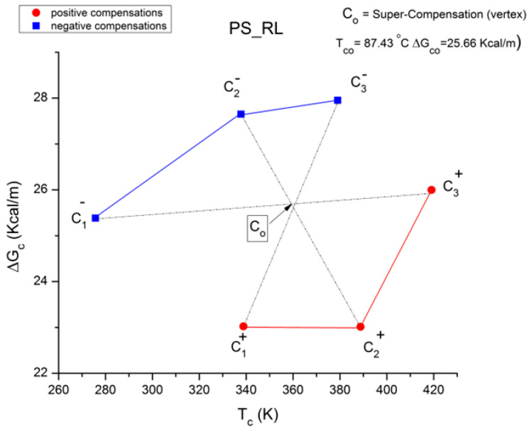
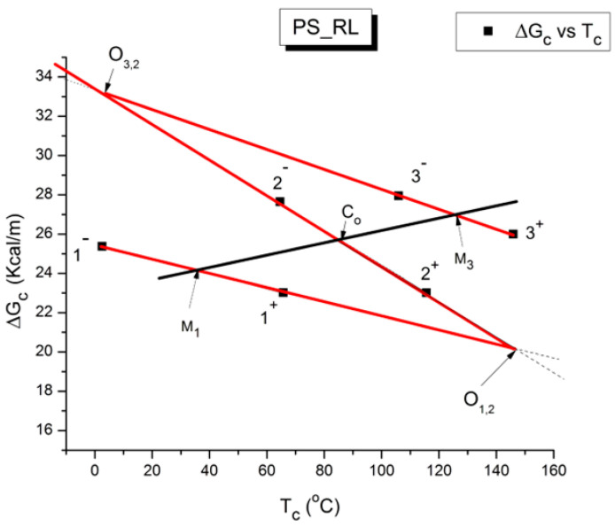
This paper addresses the author's current understanding of the physics of interactions in polymers under a voltage field excitation. The effect of a voltage field coupled with temperature to induce space charges and dipolar activity in dielectric materials can be measured by very sensitive electrometers. The resulting characterization methods, thermally stimulated depolarization (TSD) and thermal-windowing deconvolution (TWD), provide a powerful way to study local and cooperative relaxations in the amorphous state of matter that are, arguably, essential to understanding the glass transition, molecular motions in the rubbery and molten states and even the processes leading to crystallization. Specifically, this paper describes and tries to explain 'interactive coupling' between molecular motions in polymers by their dielectric relaxation characteristics when polymeric samples have been submitted to thermally induced polarization by a voltage field followed by depolarization at a constant heating rate. Interactive coupling results from the modulation of the local interactions by the collective aspect of those interactions, a recursive process pursuant to the dynamics of the interplay between the free volume and the conformation of dual-conformers, two fundamental basic units of the macromolecules introduced by this author in the "dual-phase" model of interactions. This model reconsiders the fundamentals of the TSD and TWD results in a different way: the origin of the dipoles formation, induced or permanent dipoles; the origin of the Wagner space charges and the T_g,ρ transition; the origin of the T_LL manifestation; the origin of the Debye elementary relaxations' compensation or parallelism in a relaxation map; and finally, the dual-phase origin of their super-compensations. In other words, this paper is an attempt to link the fundamentals of TSD and TWD activation and deactivation of dipoles that produce a current signal with the statistical parameters of the "dual-phase" model of interactions underlying the Grain-Field Statistics.

Keywords: TSD; TWD; amorphous state; compensations; dual-phase model; grain-field statistics; interactive coupling; super-compensations; thermal depolarization kinetics; thermal-electrical stimulation; wagner charges.

Figure 20

Variation in dN_b/dT vs. T(K) during cooling. Effect of the cooling rate. Reproduced with permission from [4], SLP Press, 1993.

Figure 21

Variation in N_b vs. T(K) during cooling. Effect of the cooling rate. Reproduced with permission from [4], SLP Press, 1993.

Figure 26

Kinetics study of N_b(t) on annealing at two temperatures (T₁ = 313.90 K, T₂ = 305.51 K). Reproduced with permission from [4], SLP Press, 1993.

Figure 27

Study of n_tb kinetics Δ_e = 250, Δ_m = 9250, υ_m = 10¹¹. Annealing at T = 313.896 K. Reproduced with permission from [4], SLP Press, 1993.

Figure 28

Arrhenius plot of Ln(k_x) vs. 1000/T. Δ_m = 9250, υ_m = 10¹¹, Δ_e = 300. Reproduced with permission from [4], SLP Press, 1993.

Figure 29

TSD depolarization curve obtained for ABS polarized at −40 °C (arrow) for 1.5 min under 200 V/mm of sample thickness. This illustration is the output curve of the TSC/RMA spectrometer by Solomat Instrument (1989). Reproduced with permission from [4], SLP Press, 1993.

Figure 40

Relaxation map in the Eyring plane for a very slowly cooled compression-molded polystyrene sample with almost no pressure during cooling. The sample is called PS_VA in subsequent figures. The slope and intercept of the elementary deconvoluted relaxations provide the enthalpy and entropy values in Table 1. The data are analyzed in Figure 41, Figure 56, and Figure 57. Reproduced with permission from [4], SLP Press, 1993.

Figure 41

Compensation search in the EE plane for the data of Figure 40. The numbers near the data relate to the row position in Table 1. Reproduced with permission from [4], SLP Press, 1993.

Figure 43

Compensation search in the EE plane for the PS_RL sample of Figure 42. The analysis appears complex. The numbers near the data (black squares) are the row numbers in Table 2 corresponding to the T_p value (shown in the inset) during TWD. For a simple amorphous state, such an EE plot has two straight lines going through the data, a positive and a negative compensation line intersecting at T_g, but we cannot represent such a simple solution since compensation lines should join consecutive increasing or decreasing T_p points for positive or negative compensations, respectively. The finding of the true positive and negative compensation lines for this complex situation is shown in Figure 45 and Figure 46.

Figure 44

Compensation search in the EE plane (Enthalpy vs. Entropy) plane for PS_RL to find the compensation(s) in Figure 42. Several positive and negative compensations emerge from what initially looked complex (in Figure 43). The down arrows indicate positive compensations, whereas the up arrows indicate negative compensations.

Figure 45

Compensation search in the EE plane for PS_RL showing the positive compensation results only (lines joining successive T_p points with increasing values of ΔS_p and ΔH_p). The 3 positive compensation lines converge to a “super-compensation” point (whose y-coordinate is ΔS_sc(+) = 0) for option 1. For option 2, with 4 compensations, only 3 of them super-compensate. The analysis for the negative compensations is illustrated in Figure 46.

Figure 46

The compensation search in the EE plane for PS_RL showing only the negative compensation results of the analysis conducted in Figure 43. In option 2, the 4 negative compensation lines converge to a single point, a super-compensation point whose ΔH_pc(−) = 18.8 Kcal/m and Δ_Spc(−) = −23 cal/m-K. For option 1, with C₃− = (14,15,16,17)), there are only 3 negative compensations and the super-compensation is defined with less confidence (r² = 0.988). For option 2, with C₃− and C₄− defined in the inset, the convergence to a super-compensation is established with confidence (r² = 0.9987).

Figure 47

Schematic reconstruction for PS_RL of the compensations of the spectral lines in Figure 42 following the compensation search results of Figure 45 and Figure 46. This graph shows the full Debye spectral lines for the 3 positive compensations (with F, D, and B indicating the aligned compensation points); the spectral lines for the negative compensations are only visible for the lower T_p compensation points (E and C) and not for compensation point A.

Figure 48

Plot of ΔG_c vs. T_c for the 6 compensations in Table 4. Red, bottom curve: positive compensation points; blue, top curve: negative compensation points.

Figure 49

Possible correlations between the compensation points across polarities.

Figure 50

Other possible correlations between the compensation points across polarities. See the text.

Figure 51

Z-structure-type correlations between the compensation points across polarities.

Figure 52

Z-structure (ZIM) compensation network for PS_RL.

Figure 53

The two compensation lines, “positive” (points 3 to 9 at the top) and “negative” ((9,10,11) at the bottom) define the behavior of amorphous phase “2”. Their intersection occurs at T_g, providing ΔH_g and ΔS_g.

Figure 54

ΔG_p vs. T_p for PS_RL. The dashed red line is the expected behavior for a stable sample (with no internal stress before polarization). ΔG_p = ΔH_p – Tp(K)ΔS_p.

Figure 55

This figure illustrates the superposition of the graphs in Figure 52 and Figure 54. The ZIM structure of Figure 52 is here visible as red dashed lines. The blue line has the same slope as the dashed line of Figure 54 but is shifted by regression to fit the square data points. See the text.

Figure 65

Normalized compensation search of Ln(υ_x/υ_m) vs. (Δ_x − Δ_m) for Δ_m = 9500, υ_m = 10¹¹. Effect of varying Δ_e. Here, Δ_e decreases from Δ_e = 400, at the left, to Δ_e = 5, at the far right. Notice that Δ_e =0 corresponds to Δ_x = Δ_m and υ_x = υ_m. Reproduced with permission from [4], SLP Press, 1993.

Figure 66

Influence of Δ_e on Δ_x and Ln υ_x using the normalized variables. This is the same graph as in Figure 65, except that Δ_m = 8,750 and υ_m = 10¹². The point (x) for (Δ_x − Δ_m) = −268 appears to be off the line. See text. Reproduced with permission from [4], SLP Press, 1993.

Figure 67

Similar to Figure 65, except that Δ_m = 9250 and Δ_e ranges from 900 to 5 as the index of the points continuously decreases from point #12 to point #1 in Table 6. What may appear chaotic can be considered a network of interlaced positive and negative compensation lines (Figure 68) for Ln(υ_x) vs. Δ_x. Reproduced with permission from [4], SLP Press, 1993.

Figure 68

Same compensation search as in Figure 67 but without the normalization of the axes by Δ_m, υ_m. This presentation of the results makes the analogy of the compensation at Δ_e variable in Figure 68 with that of −Ln τ_o vs. ΔH at T_p variable in depolarization compensation searches more apparent.

Figure 69

Variation of Ln(υ_x/υ_m) against Δ_e at υ_m and Δ_m constant, for the data of Figure 67 (Table 6). Reproduced with permission from [4], SLP Press, 1993.

Figure 70

Variation of (Δ_x − Δ_m) against Δ_e at Δ_m and υ_m constant, for the data of Figure 67 (Table 6). Reproduced with permission from [4], SLP Press, 1993.

Figure 1

Description of the steps involved in a TSD experiment (polarization, cooling, annealing, and heating) resulting in the output (a depolarization current vs. temperature) by thermal stimulation. Reproduced with permission from [4], SLP Press, 1993.

Figure 2

(a). Depolarization current vs. temperature during the thermal stimulation heating stage of Polyamide 12. (b). Depolarization current vs. temperature during the thermal stimulation heating stage for a polarization temperature near the β-transition of an amorphous polymer. Reproduced with permission from [4], SLP Press, 1993.

Figure 3

Description of the steps involved in a TWD experiment to thermally deconvolute a global TSD peak into its elementary Debye components and determine the interactive coupling between the relaxation modes. Reproduced with permission from [4], SLP Press, 1993.

Figure 4

Current of depolarization vs. T for a TWD experiment. The polymer is PMMA. Reproduced with permission from [4], SLP Press, 1993.

Figure 5

Effect of changing the polarization temperature T_p in a TWD experiment, indicated by the arrow, on the current of depolarization vs. T plot. Reproduced with permission from [4], SLP Press, 1993.

Figure 6

Conversion of the output in Figure 4 to an Arrhenius spectral line. The bottom axis is the Arrhenius scale, 1/T (K), in descending numbers; the top axis is the temperature in °C. The y-axis is the log of the relaxation time for the mode isolated by TWD at T_p. Reproduced with permission from [4], SLP Press, 1993.

Figure 7

Relaxation map in the Arrhenius plane of all the relaxation modes isolated by TWD at various T_p, as shown in Figure 5. Reproduced with permission from [4], SLP Press, 1993.

Figure 8

Illustration of the effect of various mechanical treatments of the melt during molding on the aspect of the relaxation map obtained by TWD of the glasses produced. Reproduced with permission from [4], SLP Press, 1993.

Figure 9

Response of a dielectric material to an AC voltage field. A Cole–Cole plot (top) consists of a plot of ε″(f) vs. ε′(f) at a given T; a frequency map is shown at the bottom for ε″(f,T). Such plots can be calculated from the TSD/TWD response. Reproduced with permission from [4], SLP Press, 1993.

Figure 10

Relaxation map in the Arrhenius plane illustrated for PMMA (limited to T_p < T_g). The spectral lines obtained at various T_p converge at a compensation point. The coordinates of the compensation point are assumed to reflect the state of the amorphous phase due to the interactive coupling between the relaxation modes. Reproduced with permission from [4], SLP Press, 1993.

Figure 11

The “Z structure” of the T_g transition with a positive compensation of the Debye relaxations for T_p < T_g and a negative compensation for T_p > T_g. The last relaxation of the interactive coupling network is the horizontal relaxation passing through the negative compensation point (log τ_c− = 4.77), which corresponds to T_p = T_LL (ΔS_p = 0), and the 1st relaxation of the interactive coupling network is the horizontal line passing through the positive compensation point (log τ_c+ = −0.77), which corresponds to T_β. Reproduced with permission from [4], SLP Press, 1993.

Figure 12

Compensation Search to determine the positive and negative compensation lines from a ΔG vs. T relaxation map. Reproduced with permission from [4], SLP Press, 1993.

Figure 13

Sketch of a covalent conformer (Figure 1.2 of [10]), after Flory’s three-bond unit [19]. Reproduced with permission from [4], SLP Press, 1993.

Figure 14

Variation in dN_b/dt during cooling (q = −1) Δ_m = 9250, Δ_e = 250, υ_m = 10¹¹, B_o = 1000, T_o = 400 K. The 1st peak observed (at ~ 300 K) is influenced by the value of the pair (Δ_m, υ_m), whereas the 2nd peak, only visible by a small hump at T~200 (K) in this Figure, is the reflection of the value of Δ_e on the kinetics. Reproduced with permission from [4], SLP Press, 1993.

Figure 15

Dual-split kinetic simulation. Variation in dN_b/dt during cooling (q = −1). Δ_m = 9250, Δ_e = 250, υ_m= 10¹¹, B_o = 1000, T = 400 (K). Reproduced with permission from [4], SLP Press, 1993.

Figure 16

Dual-split kinetics (cooling at q = −1). Compare the simulations of the dual-split kinetics (DSK = EKNETICS) in Equations (6)–(8) and classical kinetics in Equations (1)–(3) using the same parameters (Δ_m = 9250, Δ_e = 250, υ_m = 10¹¹, B_o = 1000, T = 400 (K)). Reproduced with permission from [4], SLP Press, 1993.

Figure 17

Variation in the energetic kinetic variables n_tb and n_tf during cooling (q = −1). Δ_m = 9250, Δ_e = 250, υ_m = 1011. Reproduced with permission from [4], SLP Press, 1993.

Figure 18

Variation in n_tb and n_cgb during cooling. Δ_m = 9250, Δ_e = 250, υ_m = 10¹¹. Reproduced with permission from [4], SLP Press, 1993.

Figure 19

Variation in I_b, I_f, and I_ds with temperature (cooling curves). Reproduced with permission from [4], SLP Press, 1993.

Figure 22

Compare N_b during heating and cooling. Δ_m = 9250, Δ_e = 250, υ_m = 10¹¹, B_o = 1000. Reproduced with permission from [4], SLP Press, 1993.

Figure 23

Compare n_tb during heating and cooling. Δ_m = 9250, Δ_e = 250, υ_m = 10¹¹, B_o = 1000. Reproduced with permission from [4], SLP Press, 1993.

Figure 24

Phase plot of dN_b/dt vs. dn_tb/dt for a cooling step (q = −1) followed by a heating step (q = +1), both steps followed by arrows 1 and 2 on the curve, respectively. Δ_m = 9250, Δ_e = 250, υ_m = 10¹¹, B_o = 1000, T = 400 K. Reproduced with permission from [4], SLP Press, 1993.

Figure 25

Variation in N_b(t) on annealing at two temperatures (T₁ = 313.90 K, T₂ = 305.51 K). Reproduced with permission from [4], SLP Press, 1993.

Figure 30

The TSD depolarization curve obtained for PET showing the T_g and T_gρ peaks. The T_gρ manifestation can be correlated to the free volume content in the material. Reproduced with permission from [4], SLP Press, 1993.

Figure 31

The TSD depolarization curve obtained for PC showing the T_g and T_gρ peaks. The arrow indicates the temperature of polarization. Reproduced with permission from [4], SLP Press, 1993.

Figure 32

TSD depolarization curve obtained for an oriented compression-molded PS sample showing T_g and two other peaks above T_g. Reproduced with permission from [4], SLP Press, 1993.

Figure 33

TSD depolarization curve obtained for a mechanically pressurized and vibrated PC sample during its compression molding showing the compensation between the T_g and T_gρ peak intensity when the sample is annealed due to the repeated polarizations performed above T_g on the same sample. Reproduced with permission from [4], SLP Press, 1993.

Figure 34

Variation with the thermo-mechanical history of the molded PS of the T_gρ peak perceived as a WLF curve in the Arrhenius plane after conversion using Bucci’s equation [14,15]. Reproduced with permission from [4], SLP Press, 1993.

Figure 35

TSD depolarization curve obtained for a vibrated oriented compression-molded PS sample (rheomolded) after polarization at T_p = 160 °C showing T_g and two other peaks above T_g. Reproduced with permission from [4], SLP Press, 1993.

Figure 36

Variation in the position of the T_gρ peak with T_p for a static (no vibration) oriented compression-molded PS sample, exhibiting the T_LL transition at 160 °C. Reproduced with permission from [4], SLP Press, 1993.

Figure 37

The DSC trace comparison of two PS samples: the reference at the top is a compression-molded general-purpose PS. The bottom trace gives the response for a rheomolded sample, compression-molded, and vibrated at the same time while cooled. The cooling conditions were the same for both samples. Reproduced with permission from [4], SLP Press, 1993.

Figure 38

Schematic description of a compensation search in the EE plane to characterize the amorphous phases across their respective T_g for a two-phase system, typically a block polymer. Reproduced with permission from [4], SLP Press, 1993.

Figure 39

Schematic description of a compensation search in the EE plane to characterize the amorphous phase across T_g for a single-phase system, typically an amorphous homopolymer. Reproduced with permission from [4], SLP Press, 1993.

Figure 42

Relaxation map in the Eyring plane for a “rheomolded” compression-molded PS sample designated PS_RL. The sample is pressurized and vibrated during fast cooling in the mold. Reproduced with permission from [4], SLP Press, 1993.

Figure 56

ΔS_p vs. T_p for PS_RL.

Figure 57

Revised Figure 41 considering points (4,5,6) forming a positive compensation. Additionally, note that the intercept of lines (1,2,3,4)⁻ and (4,5,6)⁺ is point 4, which is located on the ΔS = 0 horizontal line, perhaps indicating that the end of a negative compensation occurs for a T_p value for which ΔS = 0. Point 6 starts a new compensation for a T_p value that corresponds to ΔG_g = ΔG_c. See text.

Figure 58

New understanding of the PS_VA thermo-kinetics results of Table 1. Compare to the network of compensations of PS_RL in Figure 48. The negative compensations are positioned here below the positive compensation, which is the opposite of what is seen in Figure 48.

Figure 59

Speculative network of compensation using the geometrical criteria from the analysis of PS_RL to find the “missing” compensation points due to a lack of experimental points at lower and higher T_p. The known values are in colored text, the extrapolated ones are in black text and with an interrogation point beside them. Compare to Figure 52 for PS_RL.

Figure 60

ΔS_p vs. T_p for PS_VA. Compare to Figure 56 for PS_RL. There is only Tg visible, and the peak of ΔS_p at T_g is the expected aspect for stable samples. The 4 points at the lower T_p end correspond to the negative compensation branch of the peak expected to be found for T_g(−): a hyperbolic fit could be used to fit those points and determine the value of the T_p asymptote equal to T_g(−).

Figure 61

ΔG_p vs. T_p (C) for sample PS_VA. Compare to Figure 54 for PS_RL. For this slowly cooled sample, the mechanical history resulting in internal stress appears to have vanished since the ΔG_p vs. T_p returns to a straight line with a slope of 0.07 cal/m-K, as expected for stable samples. The explication of the deviation of 2 of the higher T_p points remains uncertain.

Figure 62

Dual-split kinetic simulation (solution of Equations (6)–(8) of Section 1.2) for Δ_m = 9250, υ_m = 10¹¹, Δ_e = 700. Cooling simulation from T_o = 515 K with the cooling rate q = −1. The two curves designate the kinetic rates for the population of n_tb and N_b. T_LL is the “dissipative“ temperature defined by the onset of an increase in dN_b/dt. Upon cooling, T_LL is the temperature at which the classical kinetics convert to EKNETICS. Upon heating (Figure 22 and Figure 23, and also Figure 37), T_LL is the temperature ending the EKNETICS now returning to classical kinetics. Reproduced with permission from [4], SLP Press, 1993.

Figure 63

Ln υ_x vs. Δ_x for Δ_m = 9250, υ_m = 10¹¹ and Δ_e variable. Reproduced with permission from [4], SLP Press, 1993.

Figure 64

Effect of Δ_e for various Δ_m and υ_m values. Note that Δ_e decreases from left to right (from 150 to 5). Reproduced with permission from [4], SLP Press, 1993.

References

1. Lacabanne C. Ph.D.Thesis. Université Paul Sabatier; Toulouse, France: 1974.
1. Vanderschueren J. Ph.D.Thesis. University of Liege; Liège, Belgium: 1974.
1. Van Turnout J. Thermally Stimulated Discharge of Polymer Electrets. Elsevier; Amsterdam, The Netherlands: 1975.
1. Ibar J.P. Fundamentals of Thermal Stimulated Current (TSC) and Relaxation Map Analysis (RMA) SLP Press; Stratford, CT, USA: 1993.
1. Ibar J.P. Dual-Phase Depolarization Analysis. Interactive Coupling in the Amorphous State of Polymers. de Gruyter; Berlin, Germany: Boston, MA, USA: 2022.
LinkOut - more resources