Experience-dependent reorganization of inhibitory neuron synaptic connectivity

Abstract

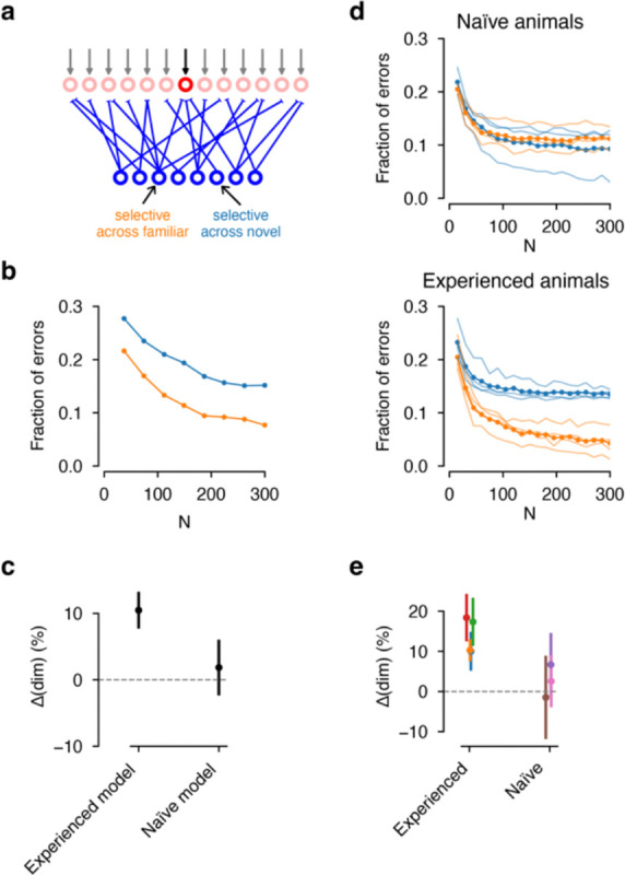
Organisms continually tune their perceptual systems to the features they encounter in their environment^1-3. We have studied how ongoing experience reorganizes the synaptic connectivity of neurons in the olfactory (piriform) cortex of the mouse. We developed an approach to measure synaptic connectivity in vivo, training a deep convolutional network to reliably identify monosynaptic connections from the spike-time cross-correlograms of 4.4 million single-unit pairs. This revealed that excitatory piriform neurons with similar odor tuning are more likely to be connected. We asked whether experience enhances this like-to-like connectivity but found that it was unaffected by odor exposure. Experience did, however, alter the logic of interneuron connectivity. Following repeated encounters with a set of odorants, inhibitory neurons that responded differentially to these stimuli exhibited a high degree of both incoming and outgoing synaptic connections within the cortical network. This reorganization depended only on the odor tuning of the inhibitory interneuron and not on the tuning of its pre- or postsynaptic partners. A computational model of this reorganized connectivity predicts that it increases the dimensionality of the entire network's responses to familiar stimuli, thereby enhancing their discriminability. We confirmed that this network-level property is present in physiological measurements, which showed increased dimensionality and separability of the evoked responses to familiar versus novel odorants. Thus, a simple, non-Hebbian reorganization of interneuron connectivity may selectively enhance an organism's discrimination of the features of its environment.

Extended Data Figure 1 |. Validation of synapse inference method

a, Top: Simplified diagram illustrating the architecture of the mouse olfactory system. Bottom: Nissl stain from Allen Brain Atlas. Yellow marks, probe shanks drawn to scale. Green shading, anterior piriform cortex. The cell dense layer 2 and layer 3 span the four shanks of a Neuropixels 2.0 probe. b, Representative examples of CCGs corresponding to pairs identified by Dyad as being monosynaptically connected via an excitatory (left) or inhibitory (right) synapse. c, Dyad architecture. Dyad consists of two convolutional layers followed by three fully-connected layers and it was trained to classify pairs as connected based on their correlogram (see Methods). The convolutional layers enabled Dyad to learn the distinctive features of cross correlograms of monosynaptically connected pairs, while maintaining flexibility, within a narrow window, with respect to the exact latency of the peak that characterizes such correlograms. d – g, Validation of Dyad on Synthetic ground-truth data. d, Illustration of the model used to generate synthetic data (see Methods). e, Left: Precision of Dyad compared to previously-published methods in detecting monosynaptically connected pairs in simulated ground truth data (see Methods and full precision-recall curves in Fig. 1d-bottom), when the detection threshold is set to obtain 70% recall. Right: Precision at 70% recall for different values of connectivity density of the simulated ground truth network. The left and center panel show results obtained for a simulated network with 2.5% connection probability. Previously published methods: English (peak-detection algorithm); Das (GLM-based inference); Endo (deep learning approach). f, Precision (left) and recall (right) at a fixed threshold, as a function of simulation time in a simulated network with 2.5% connection probability. For all the other panels, 14,400 seconds of simulated time were used. g, Precision-recall curves for excitatory (left) and inhibitory (right) connections, for various levels of connectivity density, averaged over three network realizations and three random subsampling of the single units. The connection probability in the legend indicates the connection probability of excitatory (left) or inhibitory (right) connections. h, Identification of E and I neurons. For all recorded single units, we plot their firing rate across the whole session, against their waveform width (trough-to-peak, see inset). The red dashed line in the right panel indicates the boundary used to classify single units as E or I (see Methods): single units that lie to the left of it are classified as I and those that lie below are classified as E. This boundary is defined by a nonlinear SVM trained using the labels shown in the right and bottom panels (see Methods). The colored circles overlaid indicate whether at least one excitatory (left, red circles) or inhibitory (right, blue circles) connection was found outgoing of that single unit. Points were jittered along the x-axis to ease visualization. The dashed cyan box illustrates the definition of I neurons used to estimate Dyad’s precision in inferring excitatory synapses: firing rate > 5 spikes per second, trough-to-peak < 0.5 ms (see Methods). Yellow-filled circles indicate putative false positives (see Methods). i, Dependance of connection probability on firing rate, separately for E-to-E, E-to-I, and I-to-E neuron pairs. The firing rate was calculated over the course of the entire session, either for the presynaptic neuron of the pair (left column), the postsynaptic neuron (right column), or the geometric mean of the two (right column). j, Assessing Dyad’s precision using CCG peaks on anticausal side (see Methods). Top: asymmetric peaks skewed to the right in the anti-causal window (top) are considered false positives. Bottom: Detection rate (connections found divided by the total number of pairs) of Dyad in the anticausal window compared to causal one, for excitatory (left) and inhibitory (right) connections. Dyad detected 12 excitatory and 7 inhibitory false positives out of 1,490,149 total pairs (N = 2 mice). k, Assessing the prevalence of disynaptic chains (see Methods). Red dashed line: probability of triplet motifs, in which the first single unit of a disynaptic pathway also connects to the last; gray histogram: the same connection probability for a null model in which connections are shuffled while preserving the in- and out degrees of individual single units; blue dashed line: median of the null model. l, Distribution of efficacies for all excitatory synapses detected by Dyad. The efficacy is defined as the probability of the postsynaptic single unit emitting a spike between 0.5 and 3 milliseconds after the presynaptic spike. Red dashed line: median. m, Cumulative fraction of connected pairs, against the distance between the single units in the pair. n, Left: Number detected excitatory inputs to, and excitatory outputs from, E neurons. In this plot the points were jittered to ease the visualization. Right: incoming excitatory connections against detected outgoing inhibitory connections in I neurons. r, P: Pearson’s correlation coefficient and corresponding P-value. Top, distributions of the number of excitatory inputs to (right), and inhibitory outputs from (top) these I neurons. o, Connection counts for full-cell reconstructions of neocortical (inhibitory) basket cells imaged under large-scale serial electron microscopy^,. The number of excitatory inputs onto a basket cell is strongly correlated with its number of inhibitory outputs onto excitatory neurons (Pearson’s r = 0.79, P < 10⁻¹⁰, N = 57 neurons from one mouse). r, P: Pearson’s correlation coefficient and corresponding P-value.

Extended Data Figure 2 |. Odor-evoked response properties of E and I neurons in the piriform

a–d, Response properties of an example E neuron. a, Spike time autocorrelogram. b, Mean action potential waveforms recorded on the 8 electrode sites of the probe that detected the highest-amplitude signals. c, Top: spike raster of odor-evoked responses, aligned to the valve opening time. Trials are sorted by odorant stimulus then trial number, and spikes (markers) are colored according to odorant stimulus. Bottom: Peristimulus time histograms, same color scheme as above. d, Trial-averaged, baseline-subtracted evoked firing rates in a two-second window following stimulus onset, sorted in descending order. e, Distribution of the percentage of spikes violating the refractory period (inter-spike interval < 1.5 msec, see Methods) across the population of E neurons. f, Heatmap showing z-scored trial-averaged stimulus-evoked responses of 500 randomly-selected E neuron-odor pairs, sorted from high increase in evoked rate (red) to high decrease in rate (blue). The z-score was computed based on a 2-sec window preceding stimulus onset to estimate the mean and standard deviation. The black bar indicates the time window in which odors are presented. g, Fraction of E neurons responsive to a given number of odor stimuli. Responsiveness was assessed using a paired Wilcoxon signed-rank test between the number of spikes in the two seconds preceding and following odor presentation, with a threshold of 10⁻⁴ on the P-value. h, Same as g, but separating neurons whose activity increased after odor delivery (red) from those whose activity decreased (blue). i, Cumulative distribution of spontaneous (black) and stimulus-evoked (green) firing rates; medians indicated in dashed lines. The stimulus-evoked rate was computed using a 2-sec window following stimulus onset. j–m, Same as a–d, but for an example I neuron. n–r, Same as e–i, but for the population of I neurons. s, Odorants employed and their molecular structure. t, Cumulative distributions of lifetime sparseness, for E and I neurons. In panels t–y, red and blue correspond to E and I neurons, respectively. See Methods for details about how each statistic was computed. u, Population sparseness. The box indicates the 1^st and 3^rd quartile (horizontal line: median), and the whiskers indicate the full range of the data. Each marker corresponds to one odor stimulus and one animal. v, Cumulative distributions of the coefficient of variation of single-neuron responses across trials. w, Cumulative distributions of the standard deviation of trial-averaged responses. x, Cumulative distributions of maximum selectivities. For each neuron-odor pair, the selectivity was defined as the average one-vs-one classification performance on a trial-by-trial basis. The maximum selectivity was obtained for each neuron by taking the maximum across odors. y, Cumulative distributions of signal correlation, for E/E, E/I, and I/I pairs.

Extended Data Figure 3 |. Like-to-like connectivity and spatial structure in the piriform cortex

a–c, Connection probability as a function of signal correlation, as in Fig. 2b, separately for a, (E-to-E, reproduced from Fig. 2b to permit comparison), b, E-to-I, and c, I-to-E. d–f, Connection probability as a function of distance between the pair, separately for E-to-E (d), E-to-I (e) and I-to-E (f) connections. Pairs were divided into 10 distance bins so that each bin included the same number of pairs. Markers: connection probability in each distance bin, error bars: 95% confidence intervals obtained via bootstrapping; dashed lines: double exponential fit to the binned data. To assess whether the spatial structure we found is consistent with previous findings, we fixed the spatial scale of one exponential to 2 mm, as reported in prior measurements over longer distances^,. For I to E connections, the fit returned zero for the coefficient corresponding to the 2mm-wide exponential, indicating that the spatial is best fit by a single exponential. This was not the case for E to E and E to I connections, indicating that our findings are compatible with previous reports, and capture an additional, fast decay component that was not resolvable by the methodology in previous reports. g,h, Signal correlation as a function of distance between the pair, separately for E/E (g) and E/I (h) pairs. Pairs were separated in 40 equally spaced bins and for each bin the median across pairs of the signal correlation was measured. Dashed lines indicate an exponential fit to the binned data, with spatial scale reported as λ in the figure. r and corresponding P-values indicate Pearson’s correlation coefficients of the non-binned data. i–k, Connection probability as a function of signal correlation for a null model that preserves the spatial structure of the piriform (see Methods), for E-to-E (i), E-to-I (j), and I-to-E (k) connections. Blue dashed lines and shading indicate logistic fits and 5th and 95th percentile of the fit to such null model. Black dotted lines and shading are reproduced from a-c to permit comparison.

Extended Data Figure 4 |. Experience does not enhance like-to-like connectivity in the piriform cortex for E-to-E, E-to-I, or I-to-E pairs

a, Left: Diagram of the apparatus for familiarization with odors and the four odorants used in that protocol. Center: Cumulative number of times that a mouse sampled the odor ports, averaged across N = 4 mice. Right: experiment timeline. Animals underwent this familiarization protocol for approximately two weeks (orange bar) followed by a single recording session to measure synaptic connectivity and odor responsiveness. During this recording the animals were presented both the four familiar odorants they had sampled in their home cage as well as four novel stimuli. b-d. Connection probability as a function of signal correlation across novel or familiar odorant stimuli separately for b, E-to-E (reproduced from Fig. 2d to permit comparison), c, E-to-I, and d, I-to-E.

Extended Data Figure 5 |. The effect of experience on the relationship between the connectivity and selectivity of I neurons

a, Connectivity maps (left) and evoked response amplitudes (right) of the three I neurons with the highest positive selectivity index, after the example shown in Fig. 3. Black circles: estimated single unit locations; red lines: incoming excitatory connections; blue lines: outgoing inhibitory connections; grey masks: the four silicon probe shanks. b, Same as a, but for the three I neurons with the highest negative selectivity index. c, Top row: In degree (left), out degree (center), and degree (right) of I neurons in experienced animals as a function of their selectivity; degrees are normalized by the number of single units in each recording to permit pooling of multiple datasets. A single unit’s selectivity was computed using a standard difference index ($S.I.=\frac{{\sigma }_F-{\sigma }_N}{{\sigma }_F+{\sigma }_N}$, where ${\sigma }_N,$ ${\sigma }_F$ are the standard deviation of the trial-averaged odor response across novel or familiar odors, see Methods). Statistics report Pearson’s correlation coefficients and corresponding P-values with respect to a null distribution in which the single unit’s selectivities and degrees were independently shuffled. The blue dotted lines show a linear fit and shaded regions indicate the 95% confidence interval of the fit. Bottom row: Same as top, but for naïve animals. Each of the dependencies we observed in experienced mice (panel c) differed significantly from those found in naïve animals (panel e): in-degree: t = 3.13 P = 1.0 × 10⁻⁶, N = 101, 88 I neurons (experienced, naïve), out-degree: t = 1.8, P = 1.15 × 10⁻³, N = 101, 88 I neurons (experienced, naïve), degree: t = 2.71, P = 1.4 × 10⁻⁵, N = 101, 88 I neurons (experienced, naïve). d, Top: cumulative distributions of S.I.s for I neurons that are high degree (> 0.015, purple), and low degree (< 0.015, green), for experienced (top) and naïve (middle) animals. Statistics result from a Wilcoxon rank-sum test. Bottom: mean S.I. and 95% confidence intervals (assuming normality) for high- and low-degree I neurons, for experienced and naïve animals. Significance was tested using the T-test (when comparing means to zero) and the Wilcoxon rank-sum test (when comparing two different single unit groups). Experienced, high degree vs zero: P = 0.0037; t = 3.14, N = 31 I neurons; low degree vs zero: P = 0.016, t = −2.50, N = 57 I neurons. High degree, experienced vs naïve: P = 0.0069; U = −0.52, N = 31, 44 I neurons (experienced, naïve). Low degree, experienced vs naïve: P = 0.055, U = 0.07, N = 57, 57 I neurons (experienced, naïve). e, Distribution of Pearson’s r correlation coefficients between SI and in degree (top), out degree (middle) and degree (bottom) obtained when considering all 70 ways to split the eight odorant stimuli in a set of “novel” and a set of “familiar” odors, in naïve mice. The black lines show Gaussian fits to these distributions, the gray dashed lines indicate the maximum r across all possible partitions, and the red dashed line indicates the r value obtained in experienced mice (same value as shown in c-top). f, Pearson’s $r$ correlation coefficients (top) and corresponding P-values (bottom) between the degree and difference index $q(x)$ of single-neuron response properties in experienced animals. $q(x)=\frac{x_{\text{familiar}}-x_{\text{naive}}}{x_{\text{familiar}}+x_{\text{naive}}}$, where $x$ can be the trial-averaged response (“response”), the standard deviation across odors of the trial-averaged response (“selectivity”), or the coefficient of variation across trials (“CV”). Bars in both panels are sorted according to $r$. The black dashed line indicates the threshold for significance after Bonferroni correction for 9 comparisons (α = 0.0055).

Extended Data Figure 6 |. Distributions of odor selectivity and degree are unaffected by experience

a, Distribution of SIs across all I neurons in all animals. b, Cumulative distributions of S.I.s for I neurons in experienced (red) and naïve (black) animals. The P-value was computed using the Kolmogorov-Smirnov test (N_naïve = 101; N_experienced = 88). c, Distributions of I neuron in degrees (left), out degrees (center), and degrees (right), each normalized by the number of single units in each recording to permit pooling across recordings. The distributions are plotted separately for naïve (black) and experienced (red) mice, and P-values are computed using the Kolmogorov-Smirnov test (N_naïve = 101; N_experienced = 88).

Extended Data Figure 7 |. Robustness of this study’s principal findings

a, Degree as a function of S.I., separately for each mouse, as in Extend Data Figure. 5c. b, Effect of varying the size of the quantification window used to compute odor responses. Left: Pearson’s correlation coefficient (blue) and corresponding P-value (black) between I neuron out degree and S.I. in experienced animals as a function of quantification window size. Grey dashed line: P = 0.05. Right: same but for in degree. In all the analyses in this study we employed a 2-second quantification window. c, Odor-evoked firing rate as a function of S.I. for all I neurons in experienced animals. d, Normalized in-degree of layer-1 interneurons and putative somatostatine-positive (SST) neurons, as a function of their selectivity index. e, Robustness of results with respect to the choice of the threshold employed to consider a pair connected. The only inclusion criteria was the threshold without any further manual curation. Top: The normalized in-degree of I neurons increases with the selectivity index, for three different values of the connectivity threshold. Bottom: Pearson’s r and corresponding P-value between selectivity index and the normalized in-degree (left) and out-degree (right), as a function of the connectivity threshold. f, g, Connection probability did not depend on the selectivity of E neurons. f, Connection probability as a function of the selectivity index of the E neuron of the pair for E-to-I (left) and I-to-E (right) neurons. g, E-to-E connection probability, as a function of either the pre-synaptic (left) or post-synaptic (right) E neuron’s selectivity.

Extended Data Figure 8 |. Odor-evoked response properties of E and I neurons in experienced animals

Throughout this figure blue indicates novel and orange familiar odors. Unless stated otherwise, all P-values were computed using a Wilcoxon rank-sum test. See Methods for details about how the other statistics were computed. a–f, Odor-evoked responses of E neurons (N = 2,672). a, Cumulative distributions of trial-averaged evoked firing rates. b, Cumulative distributions of the standard deviation of trial-averaged evoked firing rates. c, Fraction of E neurons responsive to a given number of odors in the novel or familiar set. Responsiveness was quantified by comparing the number of spikes in the two-second window after valve opening to the number of spikes in the two-second window before valve opening. A single unit was considered responsive to an odor if the corresponding P-value was smaller than 10⁻⁴. The difference between the two distributions was assessed using the Mann–Whitney U test. Although the distribution is only marginally higher for familiar odors, the effect was significant (P = 0.00182). d, Cumulative distributions of the coefficient of variation (CV) of individual E neurons across trials. e, Cumulative distributions of lifetime sparseness of individual E neurons. Although the lifetime sparseness was only marginally larger for familiar odors, the effect was significant (P = 0.00178). f, Population sparseness (see Methods) across the population of E neurons. The box indicates the 1^st and 3^rd quartile (horizontal line: median), and the whiskers indicate the full support of the distribution of sparsities across odors and animals. g-l, Same as a-f, but for the odor-evoked responses of I neurons (N = 88).

Extended Data Figure 9 |. Principal findings hold when considering only cross-shank connections

a, Example of excitatory (left) and inhibitory (right) connectivity for one dataset, as in Fig. 1e but considering only connections across different probe shanks, which are separated by 250 μm center-to-center. b, Connection probability as a function of signal correlations for E-to-E (left), E-to-I (center) and I-to-E (right) pairs, when considering only cross-shank connections. Plots and quantifications are as in Fig 2b and Extended Data Fig. 3a–c. c, Normalized in degree (left), out degree (center), and degree (right) for I neurons in experienced animals as a function of their selectivity index, when considering only cross-shank connections. Plots and quantifications are as in Extended Data Fig. 5.

Extended Data Figure 10 |. Increased variance of inhibitory input onto E neurons decorrelates their responses

a, Fraction of error of a Hebbian linear classifier, as in Fig. 4a, but showing the results for both the experienced (top, reproduced from Fig 4a to permit comparison) and the naïve (bottom) model. b, Variance across odors of the total inhibitory current onto excitatory neurons in the model, for both the experienced (left) and naïve (right) model. The variance is computed separately across novel and familiar odors, and averaged across 100 model realizations. Error bars: 95% confidence intervals for the mean variance. c, Fraction of errors of a Hebbian classifier trained on the odor responses of E neurons, as in Fig. 4d, for each individual mouse for novel (blue) and familiar (orange) stimulus set. Solid curves: mean; shaded area: standard deviation across odors and subsamples. d, Percent change in variance estimated from our electrophysiological recordings (dashed red line, see Methods), for naïve (left) and experienced (right) mice. Gray histogram: percent change in variance that the same estimation yields when connectivity is shuffled. The reported P-values are obtained with respect to this null model. e, Difference in classification performance between novel and familiar odorant stimuli (differences from panel c, averaged across N), as a function of the amount of experience (number of nose port pokes) the mouse had with the set of odors (Pearson’s r = 0.99, P = 0.014, N = 4 mice).

Figure 1 |. Reliable inference of monosynaptic connections in the piriform cortex

a, Spike waveforms of a pair of cells (black and red traces, top), aligned to the spike times of cell 1. The increased spiking probability of cell 2 after a cell 1 spike is captured in the spike-time cross-correlogram (CCG) of the pair (bottom), which measures the probability that cell 2 fires an action potential at a range of time lags relative to cell 1. For a synaptically connected pair of neurons, a presynaptic spike produces an asymmetric peak on the causal side of the correlogram, whose shape reflects the underlying excitatory postsynaptic potential: a sharp rise at short latency followed by a slower decay to baseline^–. Precise measurement of this shape requires several hours of continuously recorded spike trains (6.1 ± 0.9 hours, mean ± s.d., min = 5.3 hours, max = 7.1 hours). b, Summary of the number of recorded single units and inferred connections (and corresponding connection probabilities). E to E: 1,297 connected out of 4,107,263 total pairs from 7 recordings; E to I: 1,649 connected out of 144,056 pairs; I to E: 1,162 connected out of 144,056 pairs; I to I: 8 connected out of 5,798 pairs. c, Examples CCGs for excitatory (top) and inhibitory (bottom) monosynaptic connections identified by Dyad. The two rightmost examples correspond to reciprocally connected E-I pairs. d, Dyad validation. Top: Precision-recall curve on an in vivo ground-truth dataset with positively identified excitatory synaptic connections. Bottom: Precision-recall curve on simulated ground-truth data (see Methods) for Dyad (blue) and previously published connectivity inference methods: English (orange, peak-detection algorithm); Das (green, GLM-based inference); Endo (red, deep learning approach). These results are for a simulated network with 2.5% connection probability. e, Estimated single unit locations (black circles) and inferred connectivity excitatory (red lines, top) or inhibitory (blue lines, bottom) for one example dataset. The contour of the circle indicates whether the single unit was classified as an E neuron (red) or an I neuron (blue). f, Heatmap of normalized CCGs for all pairs connected by an excitatory (top) or inhibitory (bottom) synapse identified by Dyad. CCGs were normalized for visualization purposes. g, Peak latency as a function of distance between the pair. Black markers: mean latency ± 95% confidence intervals at 10 equally-spaced bins of distance; red dashed line: linear fit to all the connected pairs (i.e. prior to binning). r, P: Pearson’s correlation coefficient and corresponding P-value. (N = 2,946 pairs) The axon conduction velocity v was estimated from the slope of the red dashed line.

Figure 2 |. Like-to-like connectivity in the piriform is not enhanced by experience

a, Recording session timeline. The first odor stimulus (t = 0) is presented ~2 hours after the start of the recording. Eight odorant stimuli were presented in 25 blocks, in pseudorandom order in each block. Each odor was delivered for 4 seconds, with 1 minute inter-stimulus interval. After the last odor stimulus, spontaneous activity was recorded for additional ~2 hours. b, Left: probability of E-to-E connections as a function of signal correlation (see Methods). Black markers at the top show the signal correlation of connected pairs, jittered among the y-axis for visualization purposes. The heatmap at the bottom shows the density of unconnected pairs. Dotted line: logistic regression fit; shaded area: 95% confidence interval. Gray dashed line and shaded area: logistic regression on a null model obtained by shuffling odor stimulus identities independently for each E neuron. This null model was used to compute both P-values in this panel. Right: mean connection probability and 95% confidence intervals (Clopper-Pearson) of pairs in the lower and top quartiles of signal correlation (148 and 263 connected pairs in the lower and top quartile respectively, out of 577,376 pairs). c, Odor familiarization paradigm. Four odor ports (orange) were inserted into the wall of a modified homecage. Animals underwent this familiarization protocol for approximately two weeks, then recorded from as in a. The panel of odorant stimuli consisted of the four familiar odorants that were administered in the home cage along with four novel stimuli. d, Same as b, but for experienced animals and where signal correlations were computed either across novel (blue) or familiar (orange) stimuli. Significance was tested with respect to a null model in which we constructed pseudo-novel and pseudo-familiar odor sets, each containing two random odors from the novel set and two from the familiar set.

Figure 3 |. Effect of experience on the connectivity of inhibitory interneurons

a, Example I neuron in an experienced animal. Top: evoked response amplitudes for the 4 familiar and 4 novel odors (trial average ± s.e.m.); bottom: connectivity (black circles: estimated unit locations; inferred excitatory inputs: red arrows; inferred inhibitory outputs: blue arrows; blue circles: estimated position of example I neuron). b, In degree (top) and out degree (bottom) of I neurons in experienced animals as a function of the I neurons’ index (SI). Black markers: the means and 95% confidence intervals in equally-spaced bins of SI. Blue dotted line: linear fit to the individual data points (i.e. prior to binning); blue shaded region: 95% confidence interval on this fit. P-values were obtained with respect to a null model in which S.I. and in/out degrees were independently shuffled. $S.I.=\frac{{\sigma }_F-{\sigma }_N}{{\sigma }_F+{\sigma }_N}$ where ${\sigma }_N,{\sigma }_F$ are the standard deviation of the trial-averaged odor response across novel or familiar odors, respectively (see Methods).

Figure 4 |. Effect of inhibitory wiring on network function

a, Architecture of the computational model, with inhibitory neurons (blue) projecting to excitatory neurons (red). In the experienced model, inhibitory neurons selective to familiar odors form more connections than neurons selective to novel odorant stimuli. b, Fraction of errors of a Hebbian linear classifier trained to perform odor discrimination based on the responses of excitatory neurons in the model (see Methods), plotted against the number of neurons considered. The curves are averaged across 100 model realizations, 10 cross-validation folds and separately across novel (blue) and familiar (orange) odorant stimuli. c, Percent difference in dimensionality between the familiar and novel odor responses in the experienced and naïve models (see Methods). Error bars represent 95% confidence intervals across 100 model realizations. d, Same as b, but when the classifier is trained on the responses of E neurons in our recordings. Top: naïve cohort; bottom: experienced cohort. For each value of N, the fraction of errors is averaged across 200 random E neuron subsamples. Light curves indicate individual animals, dark lines are averages across animals. e, Same as c, but for the dimensionality of the E neuron odor responses in the data. Each marker indicates a different animal, with error bars indicating 95% confidence intervals computed across different random subsampling of 500 E neurons for each dataset.

References

1. Gibson E. J. Improvement in perceptual judgments as a function of controlled practice or training. Psychol. Bull. 50, 401–431 (1953). - PubMed
1. Gibson J. J. & Gibson E. J. Perceptual learning: Differentiation or enrichment? Psychol. Rev. 62, 32–41 (1955). - PubMed
1. Fahle M. & Poggio T. Perceptual Learning. (MIT Press, Cambridge, Mass, 2002).
1. Buck L. & Axel R. A novel multigene family may encode odorant receptors: a molecular basis for odor recognition. Cell 65, 175–187 (1991). - PubMed
1. Mombaerts P. et al. Visualizing an olfactory sensory map. Cell 87, 675–686 (1996). - PubMed
Publication types
LinkOut - more resources