methylGrapher: genome-graph-based processing of DNA methylation data from whole genome bisulfite sequencing

Abstract

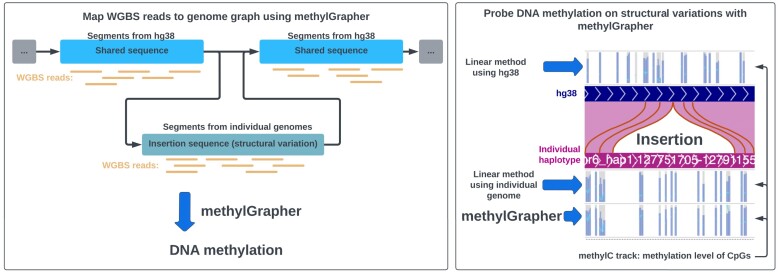
Genome graphs, including the recently released draft human pangenome graph, can represent the breadth of genetic diversity and thus transcend the limits of traditional linear reference genomes. However, there are no genome-graph-compatible tools for analyzing whole genome bisulfite sequencing (WGBS) data. To close this gap, we introduce methylGrapher, a tool tailored for accurate DNA methylation analysis by mapping WGBS data to a genome graph. Notably, methylGrapher can reconstruct methylation patterns along haplotype paths precisely and efficiently. To demonstrate the utility of methylGrapher, we analyzed the WGBS data derived from five individuals whose genomes were included in the first Human Pangenome draft as well as WGBS data from ENCODE (EN-TEx). Along with standard performance benchmarking, we show that methylGrapher fully recapitulates DNA methylation patterns defined by classic linear genome analysis approaches. Importantly, methylGrapher captures a substantial number of CpG sites that are missed by linear methods, and improves overall genome coverage while reducing alignment reference bias. Thus, methylGrapher is a first step toward unlocking the full potential of Human Pangenome graphs in genomic DNA methylation analysis.

Graphical Abstract

Figure 1.

Overview of methylGrapher's workflow. (A) The flowchart of the workflows. The middle panel illustrates the library preparation workflow. This process takes either single-end or paired-end FastQ file(s) as input. Initially, the FastQ files are trimmed using Trim Glore, deduplicated, and then fully converted prior to alignment. It is advisable to use FastQC after the trimming and deduplication steps. The left panel presents the genome preparation workflow. This workflow begins with the construction of a genome graph using the minigraph-cactus pipeline in GFA format. The lambda phage genome is incorporated as a distinct segment. Subsequently, two separate fully C-T and G-A converted graphs are generated. These can optionally have duplicated SNVs trimmed. VG Giraffe alignment indexes are then built using these two graphs. The right panel presents the alignment and methylation calling workflow. Alignments of all converted reads against all converted references were performed for non-directional libraries, and methylGrapher selects the optimal alignment for each read. If the WGBS experiment is directional, only two alignments are carried out. Using these alignments, the methylation percentage for every cytosine is calculated. After methylation extraction, read statistics are reported, and, optionally, the estimated conversion rate can be output using built-in commands. (B) A simple illustration of DNA methylation level calculation, which involves aligning reads to specific cytosines. The top half of the figure depicts a genome graph where genetic variations are represented as alternative paths in the graph. The bottom half of the figure depicts three aligned, bisulfite converted reads. After alignment, the reads are piled-up to determine how many cytosines have been converted to thymine and how many remain unchanged. (C) An example of a result table. The columns are segment ID, 0-based position on that segment, strand of the segment, cytosine context, methylated count, unmethylated count, read coverage, and methylation percentage. Here, the specific CpG with a segment ID of 10 002 was extracted from the graph in (B), and the three reads aligned to this CpG contain two CGs and one TG, thus the methylation level is estimated to be 66.67%.

Figure 2.

Performance comparison across 5 methods. Here we use sample HG00621 replicate 1 as a representative WGBS experiment which was sequenced at ∼15X. We run both methylGrapher and Bismark using default parameters three times on an identical server architecture featuring dual Intel Gold 6336Y processors and 512 GB of memory. (A) Runtime breakdown comparison across five methods over three separate runs. Here, ‘Total’ represents the overall runtime required for processing raw FastQ reads. ‘Trim’ denotes adapter-trimming, ‘Dedup’ refers to deduplication, ‘Align’ indicates the time taken for alignment including fully converting the FastQ reads, and ‘Extract’ represents the time required to extract cytosine methylation levels from the alignment file. The Y-axis displays the runtime for each step in hours. (B) Peak memory usage comparison across five methods at each step, reported from the job scheduler. The breakdown includes memory usage for ‘Trim’ (adapter-trimming), ‘Dedup’ (deduplication), ‘Align’ (alignment and conversion of FastQ reads), and ‘Extract’ (extraction of cytosine methylation levels from the alignment file). The Y-axis indicates the peak memory usage for each step in GBs. (C) The percentage of reads aligned to the reference genome is shown, with each dot representing a WGBS library. The number displayed indicates the average mapping rate. (D) The percentage of reads aligned with MapQ greater than 10, with each dot representing a WGBS library. The number displayed indicates the average mapping rate.

Figure 3.

Comparison of genome-wide analysis characteristics across the five methods. Here we use HG00621 replicate 1 as a representative in (A) and (B). All five methods generate a similar distribution of methylation. However, methylGrapher, BICUIT, and bwa-meth identify a greater number of CpG sites with higher coverage compared with Bismark and gemBS. (A) The distribution of CpG methylation levels across the five methods. Result of all methods exhibit a bimodal distribution and a similar trend in CpG genome-wide methylation distribution. The X-axis represents methylation levels from 0% to 100%, while the Y-axis indicates density in a kernel density plot. (B) The distribution of CpG coverage across all five methods. The X-axis represents CpG coverage, while the Y-axis indicates the fraction of CpG sites at specific coverage levels. (C) The number of CpG sites identified by all methods. There are 29.2 million CpGs in hg38, while the first draft of the human pangenome graph, constructed using Minigraph-Cactus for the HPRC, contains 35.8 million CpGs, as indicated by the black thin lines on top. Each bar displays the counts of CpGs identified by each of the five methods (Coverage >0), grouped by sample and replicates. The different colors illustrate CpGs called by different methods. Solid coloring indicates the count of CpGs with coverage exceeding 5X. The bar graph demonstrates methylGrapher identifies more CpG sites than linear methods.

Figure 4.

Analysis of five WGBS libraries from HPRC benchmark samples. Differences in DNA methylation calls between any methods are much smaller than differences between biological replicates. (A) The 2D histogram illustrates CpG methylation comparison between HG00621 replicate 1 and replicate 2, based on the methylGrapher results. Linear regressions are displayed in the figure. (B) The distribution of DNA methylation differences called on the same CpG between replicates. The differences are defined as ‘delta methylation’. For each CpG site between replicate 1 and replicate 2 of HG00621, delta methylation is the value of subtracting replicate 2 from replicate 1. The delta methylation is visualized using a bar graph, with CpGs categorized into 9 groups based on difference ranges (−1 to −0.35, −0.35 to −0.25, −0.25 to −0.15, −0.15 to −0.05, −0.05 to 0.05, and so on up to 0.35–1). Approximately 73.6% of CpGs exhibit a difference of less than 0.15. (C, D) Similar to Figs. 4A and B, but the comparison examines methylation differences of common CpGs’ methylation levels between the Bismark and methylGrapher, using HG00621 replicate 1 as a representative. Approximately 96.3% of CpGs exhibit a difference of <0.15. The linear regression indicates better agreement between the methods than between replicates. (E) Pearson correlation of methylation levels between replicates on common CpG sites, with sample names on the X-axis and method names on the Y-axis. (F) Pearson correlation of methylation levels between different methods on common CpG sites, with sample names and replicate numbers on the X-axis and the method names on the Y-axis. (G) PCA on common CpGs. PCA is based on the shared CpGs identified across all samples, replicates, and methods (only including Bismark and methylGrapher here) with greater than 5X coverage. The individual methylomes were separated by sample identity, then to a much lesser degree by replicates, and had very little differences between the two methods (Bismark and methylGrapher).

Figure 5.

Improvement of methylGrapher over linear methods. Here we demonstrate that methylGrapher correctly identifies the methylome in regions with genomic variation compared with Bismark. (A) Shared and unique CpGs between the methods. The breakdown of CpG counts is as follows, from top to bottom: count of Bismark unique CpG sites, count of common CpG sites between the two methods, count of methylGrapher unique CpG sites overlap with hg38, count of methylGrapher unique CpG sites with SNV, count of methylGrapher unique CpG sites within either INDEL or SV. (B) MethylGrapher fills the gap in the inserted region. An example global view from the WashU Epigenome Browser (chr1:23 268 371–23 373 036, 7.4-kb insertion, HG00621) demonstrates that methylGrapher successfully identifies the methylome within the inserted region. The red arrow on the ruler indicates the insertion breakpoint on the hg38 coordinates, while the yellow box highlights the region that was inserted. From top to bottom: refGene track, methylGrapher result surjects to hg38 (replicate 1), Bismark with hg38(replicate 1), methylGrapher result surjects to hg38 (replicate 2), Bismark with hg38 (replicate 2), HG00621 maternal genome in comparison to hg38, methylGrapher result HSS to its maternal genome (replicate 1), Bismark with maternal genome (replicate 1), methylGrapher result HSS to its maternal genome (replicate 2), Bismark with maternal genome (replicate 2), HG00621 paternal genome in comparison to hg38, methylGrapher result HSS to its paternal genome (replicate 1), Bismark with paternal genome(replicate 1), methylGrapher result HSS to its paternal genome (replicate 2), and Bismark with paternal genome (replicate 2). Data are displayed in methylC track [42]. The height of the blue bar represents the methylation percentage, while the black line indicates the coverage. (C) MethylGrapher accurately identifies CpG sites within the pan-genome. Two close-up views from the WashU Epigenome Browser (chr1:24 009 936–24 009 998) demonstrate that methylGrapher accurately identifies CpG sites without an individualized genome, while Bismark incorrectly identifies CpG sites using hg38. On the left, a homozygous CC site in the individualized genome was misidentified as a CpG site by Bismark. On the right, a homozygous CpG site was ignored by Bismark with hg38; however, Bismark identified them in the individualized genome. From top to bottom: methylGrapher result surjects to hg38 (replicate 1), Bismark with hg38 (replicate 1), methylGrapher result surjects to hg38 (replicate 2), Bismark with hg38 (replicate 2), HG00621 maternal genome in comparison to hg38, Bismark with maternal genome (replicate 1), Bismark with maternal genome (replicate 2), HG00621 paternal genome in comparison to hg38, Bismark with paternal genome (replicate 1), and Bismark with paternal genome(replicate 2). The height of the blue bar represents the methylation percentage, while the black line indicates the coverage.

Figure 6.

Analysis of EN-TEx data with methylGrapher. (A) The number of CpG sites identified by Bismark with hg38 and methylGrapher with pangenome graph. (B) The common CpG sites identified by both methods within the insertions on haplotype 1 for spleen tissue. X-axis shows methylation levels identified by Bismark; Y-axis show methylation levels identified by methylGrapher. Linear regression is shown on upper left of the figure. (C) Similar to Fig. 6B for haplotype 2 for the same library. (D) The browser screenshot of chr6_hap1:127 829 725–127 833 860 highlights a 4.1-kb insertion on hap1 compared to hg38. The track labels indicate tissue type and the processing pipeline. Bismark (Bis) was run on hap1, while methylGrapher (mG) was run on the genome graph, with the insertion region subsequently lifted over to hap1. The height of the blue bar represents the methylation percentage, while the black line indicates the coverage. (E) The browser screenshot of chr6:92 846 930–92 846 931 (hg38 coordinates) with track labels indicating tissue type and the processing pipeline. Bismark (Bis) was run on hg38, while methylGrapher (mG) was run on the genome graph and subsequently surjected onto hg38. At the bottom, two genome alignment tracks compare hap1 and hap2 to hg38. This region displays a homozygous CG site, whereas hg38 suggests a GG site. MethylGrapher identified a CpG site that was not detected by Bismark. The height of the blue bar represents the methylation percentage, while the black line indicates the coverage. (F) The browser screenshot of chr6:71 758 350–71 758 351 (hg38 coordinates), in a similar style to Fig. 6E, shows a homozygous AG site instead of a CG site. Bismark identified a false positive in this region.

References

1. Lander ES, Linton LM, Birren B et al. . Initial sequencing and analysis of the human genome. Nature. 2001; 409:860–921. - PubMed
1. Schneider VA, Graves-Lindsay T, Howe K et al. . Evaluation of GRCh38 and de novo haploid genome assemblies demonstrates the enduring quality of the reference assembly. Genome Res. 2017; 27:849–64. - PMC - PubMed
1. Nurk S, Koren S, Rhie A et al. . The complete sequence of a human genome. Science. 2022; 376:44–53. - PMC - PubMed
1. Liao W-W, Asri M, Ebler J et al. . A draft human pangenome reference. Nature. 2023; 617:312–24. - PMC - PubMed
1. Rautiainen M, Marschall T. GraphAligner: rapid and versatile sequence-to-graph alignment. Genome Biol. 2020; 21:253. - PMC - PubMed