Gastric cancer genomics study using reference human pangenomes

Abstract

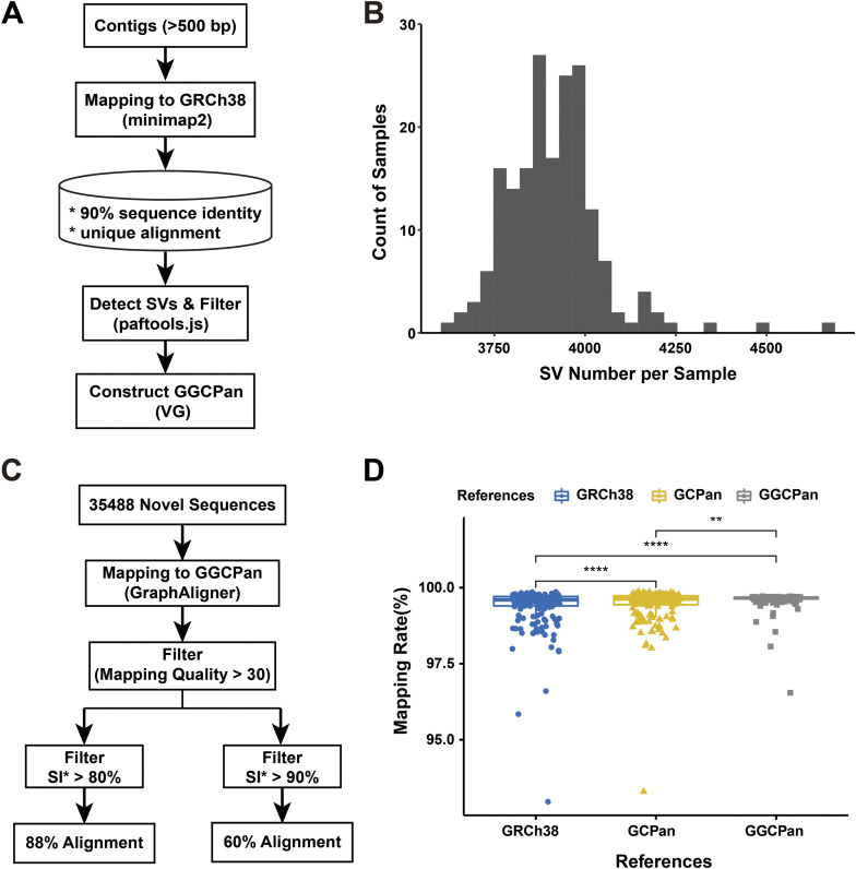
A pangenome is the sum of the genetic information of all individuals in a species or a population. Genomics research has been gradually shifted to a paradigm using a pangenome as the reference. However, in disease genomics study, pangenome-based analysis is still in its infancy. In this study, we introduced a graph-based pangenome GGCPan from 185 patients with gastric cancer. We then systematically compared the cancer genomics study results using GGCPan, a linear pangenome GCPan, and the human reference genome as the reference. For small variant detection and microsatellite instability status identification, there is little difference in using three different genomes. Using GGCPan as the reference had a significant advantage in structural variant identification. A total of 24 candidate gastric cancer driver genes were detected using three different reference genomes, of which eight were common and five were detected only based on pangenomes. Our results showed that disease-specific pangenome as a reference is promising and a whole set of tools are still to be developed or improved for disease genomics study in the pangenome era.

Figure S1.. Construction of GGCPan and comparison of mapping rate using three different reference genomes.

(A) Construction pipeline of gastric cancer graph pangenome GGCPan. (B) Histogram of the distribution of the number of SVs detected in the 185 samples. The SVs are detected by paftools.js based on minimap2 alignment results and are applied to construct the GGCPan. (C) Pipeline of non-reference sequences of GCPan aligned to GGCPan. (D) Read mapping rates of 185 gastric tumor samples on three reference genomes.

Figure S2.. Performance comparison of structural variant detection using three different reference genomes.

(A) Comparison of the performance of different tools using GRCh38 as the reference for structural variation detection using simulated data with different sequencing depths. (B) Effect of the completeness of the graph-modeled pangenome on its performance in detecting structural variants. The x-axis represents the number of samples to construct the graph-modeled pangenome. The five samples used for evaluation were excluded from the samples used to construct the five graph pangenomes. (C) Flowchart of the evaluation of different reference genomes and variant identification tools using sequencing data from the GIAB HG002 sample. Different colors represent different identification pipelines. (D) Performance evaluation results for variant identification using different reference genomes.

Figure 1.. Performance of structural variant detection using three different reference genomes.

(A) Comparison of the performance of structural variant detection using three different reference genomes in simulated data. (B) Number of somatic structural variants detected using three reference genomes in real sequencing data from 185 patients. (C) Comparison of SVs detected using GRCh38 and GGCPan in 185 patients. (D) Comparison of SVs detected using GCPan and GGCPan in 185 patients. (C, D) “+” stands for presence and “−” for absence in (C, D). (E) Enriched pathways for SV-related genes. The SVs are detected using GGCPan in 185 samples. The size of the dot represents the number of related genes included in the pathway.

Figure S3.. Comparison of structural variants in simulated data (SimuA) using GCPan and GRCh38 as the references.

(A) Overlap of GRCh38-based SVs and GCPan-based SVs in the five simulated samples (SimuA). (B) Example of insertion that was detected in GRCh38 but not in GCPan. (C) Example of deletion that was detected using GRCh38 but not using GCPan. (B, C) Gray bars in (B, C) represent the alignment of reads at this position when using GRCh38 and GCPan as the reference genomes, respectively.

Figure S4.. Population frequency of SVs detected in 185 samples using GRCh38, GCPan, and GGCPan.

Figure 2.. Comparison of numbers and types of small variants detected using three different reference genomes.

(A) Numbers of SNPs and indels detected in 185 patients with gastric tumors. Transitions and transversions are subtypes of SNPs. Insertion and deletion are subtypes of indels. (B) Numbers of different functional types of small variants (SNP, indel) detected based on the three reference genomes. (C) Left histograms: numbers and types of small variants (SNP, indel) detected in the three reference genomes in 185 patients; right histogram: types and numbers of variants in genes with mutation rates ranked top 10. The numbers at the top of the histogram represent the mutation rate. Top, middle, and bottom represent results using GRCh38, GCPan, and GGCPan as the reference genomes, respectively.

Figure S5.. There was little difference among results using different reference genomes on the detection of small variants, tumor mutation burden (TMB), and microsatellite instability (MSI).

(A) 23 genes with mutation rates differing by more than 5% in 185 samples using the three reference genomes. The y-axis represents the number of mutations per gene in 185 samples. (B) TMBs in different cohorts. The three bolded black cohorts are our gastric cancer data using three reference genomes. (C) Results of correlation tests between TMB and MSI with each phenotype. Continuous variable phenotypes (e.g., age and tumor diameter) were subjected to Spearman’s correlation test using calculated values of TMB and MSI, and other types of phenotypes were subjected to Fisher’s exact test using state values of TMB and MSI (TMB-H/TMB-L, MSI-H/ MSI-L) for Fisher’s exact test. Each grid color corresponds to the negative logarithmic value of the P-value of the correlation test. In the figure, “*” indicates that the P-value is between 0.05 and 0.01, “**” indicates that the P-value is between 0.01 and 0.001, and “***” indicates that the P-value is less than 0.001, and unlabeled positions indicate that the correlation is not significant. (D) Sample distribution of TMB-H, TMB-L and MSI-H, MSI-L/MSS in the subtypes of location, Borrmann, and Lauren.

Figure 3.. Comparison of candidate driver genes detected using different reference genomes.

(A) Candidate driver genes of gastric cancer detected using the three reference genomes. The left bar graph shows the −log₁₀(q) value of each gene, and the “*” next to a gene name indicates that the gene was determined as a driver gene using this reference genome. The q-value here stands for the significance of the gene being identified as a driver gene. The right bar graph represents the number of mutations and mutation types for each gene. The upper bar graph represents the TMB values of each sample using the three different reference genomes. (B) Enriched pathways related to the candidate driver genes. The significance threshold for enrichment analysis was P < 0.05. Numbers in parentheses represent that the gene was identified as a driver gene using the corresponding reference genome. “1” represents GRCh38, “2” represents GCPan, and “3” represents GGCPan. (C) Overlap of the candidate driver genes detected using the three reference genomes. “#” indicates that three of the four genes are related to cancers in previous studies. “##” indicates that this gene is related to cancers in previous studies. “###” indicates that this gene is related to cancers in previous studies.

Figure S6.. Correlation between the mutation status of these 24 significantly mutated genes in the cohort (yes/no mutation) and the clinical phenotype of the 185 patients.

(A) Genes significantly related to phenotypes using GRCh38. (B) Genes significantly related to phenotypes using GCPan. (C) Genes significantly related to phenotypes using GGCPan. In the figure, “*” indicates that the P-value is between 0.05 and 0.01, “**” indicates that the P-value is between 0.01 and 0.001, and “***” indicates that the P-value is less than 0.001, and unlabeled positions indicate that the correlation is not significant.

Figure 4.. Comparison of molecular subtypes, candidate driver genes, and structural variations with previous studies.

(A) Decision trees of molecular subtypes of the 185 gastric cancer patients and TCGA-STAD samples. (B) Comparison of candidate driver genes detected using three reference genomes in the 185 samples and those from two different gastric cancer cohorts (TCGA-STAD and Stomach-AdenoCA). The blue color represents the mutation rates of genes in each cohort. The gray color represents unknown mutation rate information for the gene. A circle indicates that the gene was determined to be a driver gene in this cohort. (C) Comparison of structural variants detected using GGCPan and MC, a graph pangenome constructed with healthy samples. “+” stands for presence and “−” for absence. (D) There is no overlap between the 24 candidate driver genes and the genes found to be significantly associated with the phenotype by GCPan PAV analysis.

Figure S7.. Differences in somatic copy-number variants of the four subtypes, with red color representing copy-number amplification and blue color representing copy-number deletion.

The color bar on the left represents the division of the 185 samples into four subtypes. The heatmap represents the copy-number variation for each sample. The red color represents copy-number amplification, and the blue color represents copy-number deletion.

References

1. Aaltonen LA, Abascal F, Abeshouse A, Aburatani H, Adams DJ, Agrawal N, Ahn KS, Ahn S-M, Aikata H, Akbani R, et al. (2020) Pan-cancer analysis of whole genomes. Nature 578: 82–93. 10.1038/s41586-020-1969-6 - DOI - PMC - PubMed
1. Boland CR, Thibodeau SN, Hamilton SR, Sidransky D, Eshleman JR, Burt RW, Meltzer SJ, Rodriguez-Bigas MA, Fodde R, Ranzani GN, et al. (1998) A national cancer institute workshop on microsatellite instability for cancer detection and familial predisposition: Development of international criteria for the determination of microsatellite instability in colorectal cancer. Cancer Res 58: 5248–5257. - PubMed
1. Bonneville R, Krook MA, Chen H-Z, Smith A, Samorodnitsky E, Wing MR, Reeser JW, Roychowdhury S (2020) Detection of microsatellite instability biomarkers via next-generation sequencing. In Biomarkers for Immunotherapy of Cancer: Methods and Protocols, Thurin M, Cesano A, Marincola FM (eds), Vol 2055, pp 119–132. New York, NY: Springer. - PMC - PubMed
1. Cancer Genome Atlas Research Network (2014) Comprehensive molecular characterization of gastric adenocarcinoma. Nature 513: 202–209. 10.1038/nature13480 - DOI - PMC - PubMed
1. Chen X, Schulz-Trieglaff O, Shaw R, Barnes B, Schlesinger F, Källberg M, Cox AJ, Kruglyak S, Saunders CT (2016) Manta: Rapid detection of structural variants and indels for germline and cancer sequencing applications. Bioinformatics 32: 1220–1222. 10.1093/bioinformatics/btv710 - DOI - PubMed
LinkOut - more resources