SARS-CoV-2 evolution on a dynamic immune landscape

Abstract

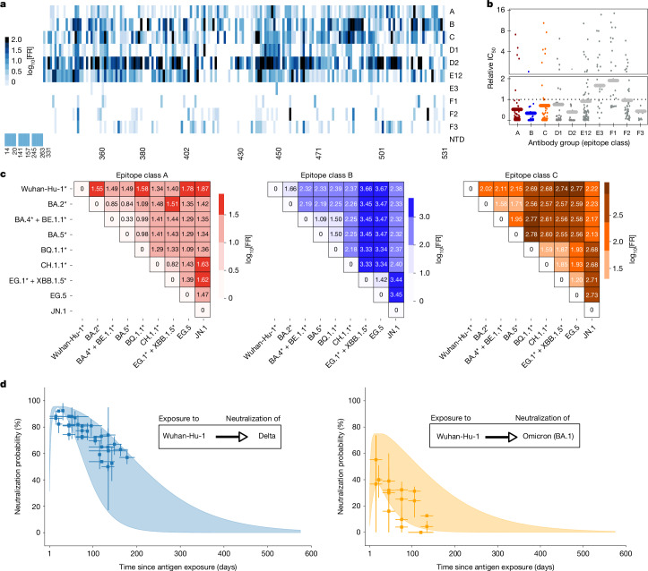
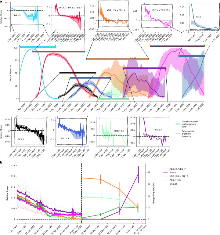
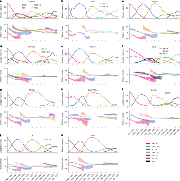
Since the onset of the pandemic, many SARS-CoV-2 variants have emerged, exhibiting substantial evolution in the virus' spike protein¹, the main target of neutralizing antibodies². A plausible hypothesis proposes that the virus evolves to evade antibody-mediated neutralization (vaccine- or infection-induced) to maximize its ability to infect an immunologically experienced population^1,3. Because viral infection induces neutralizing antibodies, viral evolution may thus navigate on a dynamic immune landscape that is shaped by local infection history. Here we developed a comprehensive mechanistic model, incorporating deep mutational scanning data^4,5, antibody pharmacokinetics and regional genomic surveillance data, to predict the variant-specific relative number of susceptible individuals over time. We show that this quantity precisely matched historical variant dynamics, predicted future variant dynamics and explained global differences in variant dynamics. Our work strongly suggests that the ongoing pandemic continues to shape variant-specific population immunity, which determines a variant's ability to transmit, thus defining variant fitness. The model can be applied to any region by utilizing local genomic surveillance data, allows contextualizing risk assessment of variants and provides information for vaccine design.

Fig. 1. Overview of data sources and data integration for modelling variant-specific immunity and fitness advantage.

DMS data are used to define fold resistance to cross-neutralization (FR; that is, factor of decreased antibody potency), conferred by mutational differences between lineages at amino acid positions relevant to antibodies of an epitope class (top right). This information is combined with the mutational profiles of the distinct lineages (top panel) to compute ‘fold resistance maps’ to cross-neutralization between any pair of lineages (x, y) for each epitope class (left, second panel from top). Asterisks (for example, XBB.1*) indicate spike pseudo groups; that is, the group of lineages with identical mutations in the spike protein (for example, identical to XBB.1, in the case of XBB.1*). Antibody pharmacokinetics (right, second panel from the top) after antigen exposure are then combined with the fold resistance maps to compute the temporal profiles of virus cross-neutralization between any pair (x, y) of immunity-inducing variant x and another variant y. Finally, these variant-resolved immune waning dynamics are combined with the timeline of infection (lower right panels) with distinct variants in any region of interest, to compute the relative number of susceptible individuals γ_y(t) (lower left) for each variant over time. The relative number of susceptible individuals γ_y(t) indicates the competitive fitness advantage of each variant: if γ_y(t) > 0, variant y has the potential to spread, and if γ_y(t) < 0, the variant will decrease in frequency and eventually vanish.

Fig. 2. Cross-neutralization and immune waning dynamics.

a, Fold resistance induced by mutational differences against antibodies of distinct epitope classes at indicated sites. b, Relative potency IC_50(DMS) of antibodies of specific epitope classes in the DMS data. The solid horizontal lines show the respective average IC_50(DMS). The dotted horizontal line marks the average across all epitope classes. c, Fold resistance to neutralization against immunity-inducing variants (on y axis) for antibodies of epitope classes A, B and C. Asterisks indicate spike pseudo groups; that is, lineages with identical mutations in the spike protein. d, Predicted neutralization probability of the Delta variant (blue range, left panel) and the Omicron variant (BA.1) (orange range, right panel) after exposure to the Wuhan-Hu-1 antigen P_Neut(t, Wuhan-Hu-1, Delta). Ranges depict minimum–maximum ranges resulting from pharmacokinetic variability. The corresponding clinical vaccine efficacy is also indicated (blue and orange markers, central estimate; vertical line, 95% confidence interval; horizontal line, range of time post vaccination as stated in the original study; see Supplementary Table 5). Source Data

Fig. 3. Dynamic immune landscape and variant dynamics in Germany.

a, Historical variant dynamics in Germany during 1 March 2022 to 1 July 2024 of spike pseudo-groups BA.2,.X BA.5.X (+ BA.4.X + BE.1.1), BF.7.X, BQ.1.1.X, XBB.1.5.X (+ EG.1.X), XBB.1.9.X, EG.5.X, JN.1.X (+ BA.2.86.X) and KP.X, where ‘.X’ denotes inclusion of the respective sublineages. Confidence intervals were computed using Wilson’s method. Insets show model-predicted relative fitness γ_y(t) (representing the relative number of susceptible individuals; coloured areas), with superimposed changes in frequency (π_y(t − 1)/π_y(t) − 1) seen in the data (solid lines). Note that the sequencing intensity changed markedly in April 2023 (vertical dashed line) as highlighted in Extended Data Fig. 3. b, Predicted variant dynamics. Left: model-predicted relative growth advantage γ_y of emerging spike pseudo-groups XBB.1.5* (+ EG.1*), XBB.1.9.X (+ EG.1.3), XBB.1.16.X, EG.5.1* and BA.2.86 (colours in key) using data until 15 April 2023 (asterisks (for example, EG.1*) indicate spike pseudo groups; that is, the group of lineages with identical mutations in the spike protein). Note that BA.2.86 was first detected on 24 July 2023 in Denmark and represents the dominating lineage (together with daughter lineage JN.1 globally, as of January 2024). Thick lines show average values, and light lines show minimum–maximum ranges resulting from pharmacokinetic variability. Right: data-derived lineage frequencies in the time after the prediction horizon (15 April 2023 to 27 July 2023). Confidence intervals (95%) were calculated using Wilson’s method with sample size n = 2,919, 500, 165 and 164 for April, May, June and July, respectively. Source Data

Fig. 4. Dynamic immune landscape and variant dynamics across the globe.

a–k, The relative abundance of major lineages when they surpass 3% relative abundance (solid lines, top) along with their model-calculated relative fitness γ_y(t) (bottom lines represent mean estimates, shaded areas represent minimum–maximum intervals resulting from pharmacokinetic variability) for Australia (a), Brazil (b), Canada (c), Denmark (d), France (e), Japan (f), Mexico (g), South Africa (h), Sweden (i), the UK (j) and the USA (k). Note that in Brazil, the lineages BQ.1.X include BE.9, and lineages XBB.1.5.X include XBB.1.18.1. Source Data

Fig. 5. Country-specific immune landscape and effects on variant success.

a, Dynamics of BA.2.12.1 in the USA (green dashed line) versus Germany (black dashed line) and Japan (red dashed line) along with the model-predicted relative number of BA.2.12.1 susceptible individuals (representing relative fitness γ_y) in the USA, Germany and Japan (green, grey and red areas, respectively). b, Dynamics of XBB.1.16 in Japan and Sweden (red and magenta dashed lines, respectively) along with the model-predicted relative fitness (red and magenta areas, respectively). c, Dynamics of BF.7 in Germany, Denmark and USA (dashed black, yellow and green lines, respectively) along with the model-predicted relative fitness (grey, yellow and green areas, respectively). d, Dynamics of endemic variant BR.2.1 in Australia (orange dashed line) versus the UK (cyan dashed line) along with the corresponding model-predicted relative fitness (orange and cyan areas, respectively). e, Model-predicted relative fitness of BA.2.86 and JN.1 in the USA, UK and Denmark (green, cyan and yellow areas, respectively) up to mid-November 2023 and variant dynamics in the following 2 months (green, cyan and yellow, respectively; error bars represent mean frequency and 95% confidence interval computed using Wilson’s method). f, Dynamics of convergently evolved lineages FE.1 in Brazil (green dashed line) versus EG.5.1 in France (purple dashed line) and predicted relative fitness (shaded areas). g, Dynamics of convergently evolved lineages GK.1 (Brazil, purple dashed line) versus HK.3 (Japan, red dashed line) along with the model-predicted relative fitness (shaded areas). Source Data

Extended Data Fig. 1. Utilization of DMS data and comparison of DMS-derived fold resistances with titer changes from mono- and polyclonal sera.

a. Theoretical binding curve of an antibody a to a wild-type epitope of SARS-CoV-2 (black line) and corresponding binding curve to an epitope that is mutated at site s (red line). The black dot and red circle mark the concentrations (x-axis) where the binding is half maximal (y-axis) for the wild type IC50_DMS(a) and mutant virus IC50_DMS(a,s) respectively. The ‘fold resistance’ (red-black dashed line) denotes the shift in the IC50, such that IC50_DMS(a,s) = FR(a, s) · IC50_DMS(a). The red square marks the DMS-measured unbound fraction (escape fraction ef(s, a)) and the upward-pointing grey arrow the concentration at which the DMS experiment was conducted. Both, IC50_DMS(a), ef(s, a) were measured in the original DMS experiment at an antibody concentration of 400 μg/mL. However, the same DMS experiment, performed with a more- (panel b.) or less (panel c.) potent antibody would yield a smaller, respectively bigger escape fraction, while the phenotypic effect FR(a, s) of the mutation s is quantitatively identical. To avoid these artifacts, we calculated FR(a, s) from the original DMS data. d. Comparison between DMS-derived fold resistances FR_x,y and fold resistances derived from neutralization assays (mono-clonal). Distinct markers show the epitope classes and distinct colors the Spike-pseudo-groups. e-g. Comparison between DMS-derived changes in neutralization and neutralization titer changes (polyclonal sera). Geometric mean change in neutralization titers for Alpha (e.), Delta (f.) and BA.2 (g.) after exposure to the Wuhan antigen are highlighted by dots (± standard deviation), whereas DMS-based model predictions are shown as a blue vertical line and were computed as outlined in^,. Raw data on neutralization titer changes^,–. h. Normalized antibody pharmacokinetics after antigen exposure. Parameters and equations given in the Methods section.

Extended Data Fig. 2. Spike-pseudo-group dynamics in Germany over the investigated time horizon.

For readability we only plot pseudo-groups (groups of lineages with identical mutation profiles in the spike protein) that appear at a frequency of > 1%.

Extended Data Fig. 3. Integration of wastewater virus loads with GInPipe’s incidence estimates and validation for Germany.

The upper panel shows the number of viral sequences per day in Germany (black bars = raw data, black line = 7-days rolling average). The middle panel depicts the estimation of the GInPipe-based minimal number of SARS-CoV-2 infected individuals per day in Germany (red area; description in the Methods) and viral load measurements from wastewater, linearly scaled to the GInPipe-based incidence (blue area). The daily reported cases are given by the black and grey dashed line. The lower panel shows the estimated under-reporting factor (ratio of incidence estimate vs. reported cases) on a log10 scale. The red line shows under-reporting estimates for GInPipe for the time with sufficient sequencing data and continuing in blue with the scaled wastewater incidence estimates. The light blue and orange points, together with the respective smoothed lines, show the under-reporting factor estimated with GrippeWeb (citizen-science) data using the virologic positivity rate approach (GW VPR) and the self-reported testing approach (GW SR). The vertical red line indicates the chosen cut date at 01. April 23, when the available sequence data declined drastically from (> 10,000 to ≤ 100 sequences/week).

Extended Data Fig. 4. Validation of genome-based incidence estimates, using data from the UK.

a. Average percentage of the population testing positive from the COVID-19 Infection Survey of the Office for National Statistics (ONS; ground truth data). Coloured lines depict the percentage for each UK constituent country. The black dashed line shows the average PCR-positivity (over all constituent countries) for the UK. b. Estimation of the SARS-CoV-2 positive population in the UK using ONS data (black line; ground truth), GInPipe’s estimate (red) scaled to the population (see Methods) and reported cases (grey), scaled to the population. A right-sided rolling sum of 10 days is applied to the reporting data and GInPipe’s estimates to approximate PCR-positivity. c. Under-reporting factor calculated as the ratio of the ONS data and the SARS-CoV-2 positive population fraction using reporting data (grey), and GInPipe’s incidence estimate (red). In line with previous work, we performed separate GInPipe-incidence reconstructions for pre-omicron vs. omicron sequences (because of different evolutionary signals^–, which are utilized in GInPipe). The pre-omicron vs. omicron estimates were then scaled and added together to compute total incidence.

Extended Data Fig. 5. Incidence reconstruction for all considered countries.

For each country, the upper panel shows the output of GInPipe (i.e., incidence correlates ϕ). The dots show the point estimates for each temporal sequence bin, while the red line depicts the smoothed incidence correlate ϕ (bandwith = 14). The black-grey line shows the reported (smoothed) SARS-CoV-2 cases for the respective country, acquired from OWID. The lower panel shows the number of sequences per day in black bars, together with the cumulative number of sequences as a grey line.

Extended Data Fig. 6. Accuracy of predictions per country and lineage (related to Fig. 4) and impact of BA.4/5 boosters.

a. Each dot represents the accuracy of a specific lineage and country combination. Accuracy is determined by partitioning the frequency curve πy into days of rising (1) and falling (−1) trends, then comparing these with corresponding predictions γ_y: If the full envelope is positive, the prediction is rising (1) if the full envelope is negative, the prediction is falling (−1): Days with negligible frequency changes or undecided predictions (envelopes with both positive and negative values) are excluded from the analysis. b. Predicted impact of bivalent (BA4/5) booster-vaccinations on the relative number of susceptibles (relative variant fitness) γ_y in Germany. Top left: Timeline of bivalent booster vaccine uptake in Germany (https://impfdashboard.de/) and average number of susceptibles (averaged with regards to the circulating ‘Spike pseudo-groups’ at the time). Remaining panels: Predicted relative fitness γ_y for major circulating variants in Germany March 2022–April 2023, without considering vaccinations (green area) and when considering both the timeline of infection and vaccinations respectively (red outlines).

Extended Data Fig. 7. Predicted impact of ≥3rd booster-vaccinations on the relative number of susceptibles (relative variant fitness) γ_y in Germany.

Top left: Timeline of booster vaccine uptake in Germany (https://impfdashboard.de/). Top right: Average number of susceptibles (averaged with regards to the circulating ‘Spike pseudo-groups’ at the time). Predicted relative fitness γ_y for major circulating variants in Germany March 2022–April 2023, without considering vaccinations (green area) and when considering both the timeline of infection and vaccinations respectively (red outlines).

Extended Data Fig. 8. Sensitivity of the developed method to diminishing data input.

We down-sampled the sequence data to 1% for Germany and superimposed model predictions for the relative variant fitness γ_y using the full dataset (green areas) vs. 1% of the data (orange areas).

Extended Data Fig. 9. Estimation of the number of infected individuals in Germany (left, red) and the UK (right, blue).

The upper panels show the estimated incidence for Germany with GInPipe and for UK using the ONS survey data over a time horizon of 13.5 months (roughly a year). The grey parts of the areas depict the officially reported cases, respectively. In the lower panels, the cumulative sum of the number of infected individuals over time are compared to the population size of the respective country, denoted by the black dashed line. The scaling factor k is given by the ratio of the population size and the sum of infected individuals within the time horizon.

Extended Data Fig. 10. Utilization of incidence correlates.

The figure shows how utilization of incidence correlates may affect relative fitness estimates γ_y (magenta dots), depending on the choice of k (k⁻¹ = estimate of the expected frequency of infection in the population over the time horizon of interest). Essentially, if k is correctly predicted (vertical dashed line), γ_y is also correctly estimated with incidence correlates ϕ(t) (in comparison to computing γ_y with actual infection numbers I(t); solid black horizontal line). If k is over- or under-estimated γ_y gets scaled (with a factor ξ). If k is underestimated, the region’s population gets under-estimated, which results in under-estimating the number of susceptibles (over-prediction of competition between variants. Note, that the qualitative results are correct in any case (inflection points γ_y = 0; variant ‘growth’ γ_y > 0 vs. variant ‘decline’ γ_y < 0).

References

1. Markov, P. V. et al. The evolution of SARS-CoV-2. Nat. Rev. Microbiol.21, 361–379 (2023). - PubMed
1. Chen, Y. et al. Broadly neutralizing antibodies to SARS-CoV-2 and other human coronaviruses. Nat. Rev. Immunol.23, 189–199 (2023). - PMC - PubMed
1. Meijers, M., Ruchnewitz, D., Eberhardt, J., Luksza, M. & Lassig, M. Population immunity predicts evolutionary trajectories of SARS-CoV-2. Cell186, 5151–5164 (2023). - PMC - PubMed
1. Greaney, A. J. et al. Complete mapping of mutations to the SARS-CoV-2 spike receptor-binding domain that escape antibody recognition. Cell Host Microbe29, 44–57 (2021). - PMC - PubMed
1. Cao, Y. et al. Imprinted SARS-CoV-2 humoral immunity induces convergent Omicron RBD evolution. Nature614, 521–529 (2023). - PMC - PubMed
Substances
Supplementary concepts