. 2025 Mar;34(3):440-456.
doi: 10.1177/09622802241304112. Epub 2025 Jan 31.

High-dimensional, outcome-dependent missing data problems: Models for the human KIR loci

Affiliations

High-dimensional, outcome-dependent missing data problems: Models for the human KIR loci

Lars Leonardus Joannes van der Burg et al. Stat Methods Med Res. 2025 Mar.

Abstract

Missing data problems are common in biological, high-dimensional data, where data can be partially or completely missing. Algorithms have been developed to reconstruct the missing values by means of imputation or expectation-maximization algorithms. For missing data problems, it has been suggested that the regression model of interest should be incorporated into the imputation procedure to reduce bias of the regression coefficients. We here consider a challenging missing data problem, where diplotypes of the KIR loci are to be reconstructed. These loci are difficult to genotype, resulting in ambiguous genotype calls. We extend a previously proposed expectation-maximization algorithm by incorporating a potentially high-dimensional regression model to model the outcome. Three strategies are evaluated: (1) only allelic predictors, (2) allelic predictors and forward-backward selection on haplotype predictors, and (3) penalized regression on a saturated model. In a simulation study, we compared these strategies with a baseline expectation-maximization algorithm without outcome model. For extreme choices of effect sizes and missingness levels, the outcome-based expectation-maximization algorithms outperformed the no-outcome expectation-maximization algorithm. However, in all other cases, the no-outcome expectation-maximization algorithm performed either superior or comparable to the three strategies, suggesting the outcome model can have a harmful effect. In a data analysis concerning death after allogeneic hematopoietic stem cell transplantation as a function of donor KIR genes, expectation-maximization algorithms with and without outcome showed very similar results. In conclusion, outcome based missing data models in the high-dimensional setting have to be used with care and are likely to lead to biased results.

Keywords: KIR genes; Missing data; expectation-maximization algorithm; haplotype reconstruction; multiple imputation; outcome dependent imputation.


Conflict of interest statement

Declaration of conflicting interestsThe author(s) declared no potential conflicts of interest with respect to the research, authorship and/or publication of this article.

Figures

Figure 1.
Figure 1.
Profile EM-algorithm with outcome for a set of loci. HTFs are updated with the profile EM-algorithm with outcome for the haplotypes (loci in reconstruction) by iterating between a weighted haplotype only profile EMalgorithm (EMprof; van der Burg et al. (2023)) and updating regression coefficients. Maximized parameters are returned as θ .
Figure 2.
Figure 2.
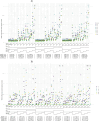
HTF estimation, scenario A. Note: Nested-loop plot of RMSEs for HTFs and HTR measure for all sub-scenarios of the proof-of-concept study without haplotype effects. Each column of points separated by vertical grid lines depicts a different set of parameters, where the lines at the bottom of the graph define these parameter sets. Each sub-scenario is analyzed by four outcome models: no-outcome (lowest line; noY), allelic model (one step; allele), forward-backward model (second step; FB), and penalized regression model (upper line; pen). The sub-scenarios differ in their added LD and ambiguities, where a step in the line corresponds to a higher value (lowest line is 0.0; highest line is 0.8). Further explanation of the nested-loop plot is given by Rücker and Schwarzer. The haplotypes plotted are a combination of gene 1, gene 2, and gene 3, with the genes in that order separated by a “ .” For visualization purposes, dots of haplotypes with a too high RMSE are replaced by a triangle and put on top of the graph. The horizontal bold black lines represent the RMSE of the population HTFs (popHTFs; with values on the left y-axis), while the bold red lines represent the HTR measure of the individual HTFs (with values on the right y-axis). The table below the graph shows mean RMSE values of these popHTFs and the HTR measures, as well as the Kullback-Leibler divergence ratios between the no-outcome model and the three outcome models. All values in the table give ranges (min–max) of values for the three sub-scenarios above. A ratio >1 indicates higher similarity of the HTFs of the outcome models with the truth than the no-outcome model. Mean RMSE values in the table have been multiplied by 100 for readability. In this plot, only the six HTs with the highest HTFs are plotted. The mean RMSE, HTR measure and table are based on all HTs, which are also displayed in Supplemental Figure S1.
Figure 3.
Figure 3.
HTF estimation, scenario 001. Note: Nested-loop plot of RMSEs for HTFs and HTR measure for all sub-scenarios of default scenario 001, containing HTF and effect size set 1. Explanation about the nested-loop plots is given in the legend of Figure 1. The horizontal bold black lines represent the RMSE of the popHTFs (with values on the left y-axis), while the bold red lines represent the HTR measure of the individual HTFs (with values on the right y-axis). The table below the graph shows mean RMSE values of these popHTFs and the HTR measures, as well as the KLD ratios between the no-outcome model and the three outcome models. All values in the table are the range (min–max) of values for the three sub-scenarios above. A ratio >1 indicates higher similarity of the HTFs of the outcome models with the truth than the no-outcome model. Mean RMSE values in the table have been multiplied by 100 for readability. In this plot only, the six HTs with the highest HTFs are plotted. The mean RMSE, HTR measure, and table are based on all HTs, which are also displayed in Supplemental Figure S3.
Figure 4.
Figure 4.
Substantive model regression coefficients, scenario 001. Note: Nested-loop plots of RMSE values for estimated regression coefficients for all sub-scenarios of default scenario 001, containing HTF and effect size set 1. Two substantive models are run with different sets of predictors: (A) only alleles as predictor and (B) all candidate list predictors as predictor. Explanation about the nested-loop plots is given in the legend of Figure 1. Here, the colored dots are either alleles (single letters) or haplotypes (combination of alleles separated by a “ ”). The gene origin of each allele is conform Table 1. The horizontal bold black lines represent the RMSE of the effect sizes, with the values displayed in the table below the graph. These RMSE values give the range (min–max) for the three sub-scenarios above. Mean RMSE values have been multiplied by 100 for readability. In this plot, only the six HTs with the highest HTFs are plotted. The mean RMSE, HTR measure, and table are based on all HTs, which are also displayed in Supplemental Figure S5.
Figure 5.
Figure 5.
HTF dissimilarity. Note: The dissimilarity between the HTFs of the no-outcome EM algorithm and the HTFs estimated with the three outcome models for different threshold values ( 1×10i for i{04,05,06,07,08,10,12,15} ) estimated with the KLD. When HTFs of two models are identical, KLD equals 0. HTFs: haplotype frequencies; EM: expectation-maximization; KLD: Kullback-Leibler divergence.

Similar articles

References

    1. Heitjan DF, Rubin DB. Ignorability and coarse data. Ann Stat 1991; 19: 2244–2253.
    1. Little RJA, Rubin DB. Statistical Analysis With Missing Data. 3rd ed. Hoboken, NJ: Wiley, 2020.
    1. Moons KGM, T. Donders RAR, Stijnen T, et al.. Using the outcome for imputation of missing predictor values was preferred. J Clin Epidemiol 2006; 59: 1092–1101. - PubMed
    1. Bartlett JW, Taylor JMG. Missing covariates in competing risk analysis. Biostatistics 2016; 17: 751–763. - PMC - PubMed
    1. Bartlett JW, Seaman SR, White IR, et al.. Multiple imputation of covariates by fully conditional specification: accommodating the substantive model. Stat Methods Med Res 2015; 24: 462–487. - PMC - PubMed

LinkOut - more resources